Table of Contents
Discuss the Outdoor Propagation Model
Discuss the Outdoor Propagation Model. Radio transmission in a mobile communications system often takes place over irregular terrain. Estimating PL(d) over a particular area requires terrain profile for propagation over irregular terrain such as
- simple curved earth profile
- highly mountainous
- obstacles: trees, building,
all models predict Pr(d) at given point or small area (sector)
- wide variations in approach, complexity, accuracy
- most based on systematic interpretation of empirical data
Some of the commonly used outdoor propagation models are:
- Longely Rice
- Durkins Model
- Okumura Model
- Hata Model
- Wideband PCS Microcell
- PCS Extension to Hata Model
- Walfisch – Bertoni Model
Longley Rice Model:
The Longley–Rice model (LR) is a radio propagation model a method for predicting the attenuation of radio signals for a telecommunication link in the frequency range of 40 MHz to 1000 GHz.
Longley-Rice is also known as the “irregular terrain model” (ITM). It was created for the needs of frequency planning in television broadcasting in the United States in the 1960s and was extensively used for preparing the tables of channel allocations for VHF/UHF broadcasting there..The Irregular Terrain Model (ITS) of radio propagation the Longley-Rice model named for Anita Longley & Phil Rice, 1968 is a general purpose model that can be applied to a large variety of engineering problems. The model, which is based on electromagnetic theory and on statistical analyses of both terrain features and radio measurements, predicts the median attenuation of a radio signal as a function of distance and the variability of the signal in time and in space.
Longley rice model is applicable to point-to-point communication systems over different kind of terrain. The median transmission loss is predicted using the path geometry of the terrain profile and the refractivity of the troposphere.
The Longley Rice Model—- A Computer Program:
In 1978, Longley-Rice model is also available as a computer program to calculate large-scale median transmission loss relative to free space loss over irregular terrain for frequencies between 20MHz and 10GHz. For a given transmission path the program takes as its input the transmission frequency, path length, polarization, antenna heights, surface refractivity, effective radius of earth, ground conductivity, ground dielectric constant, and climate. The program also operates on path-specific parameters such as horizon distance of the antennas, horizon elevation angle, angular trans-horizon distance, terrain irregularity, and other specific inputs.
Modes Of Operation:
Longley-Rice method operates in two modes
- Point-to-point Mode Prediction
- Area Mode Prediction
Point-to-point Mode Prediction:
“Longley-Rice” point-to-point model for radio propagation in the Terrain Analysis Package (TAP) when a detailed path profile is available, the path-specific parameters can be easily determined.
Area Mode Prediction:
When the terrain path profile is not available, the Longley-Rice method provides techniques to estimate the path-specific parameters.
Modifications:
There have been many modifications and corrections to the Longley-Rice model since its oroginal publication. One point modification deals with radio propagation in urban areas and this is particularly relevant to mobile radio. This modification introduces an excess term as an allowance for the additional attenuation due to urban clutter near the receiving antenna. The extra term called the Urban “Urban Factor” has been derived by comparing the predictions by the original Longley-Rice model with those obtained by Okumura.
Shortcoming:
- Does not providing a way of determining corrections due to environmental factors in the immediate vicinity of the mobile receiver.
- No consideration of correlation factors to account for the effects of buildings and foliage.
- No consideration of multipath.
Durkin’s Model:
In 1969 & 1975, Durkin propose a computer simulator for predicting field strength contours over irregular terrain. Durkin’s model Adopted by the Joint Radio Committee in the U.K. for estimation of effective mobile radio coverage areas.
- predicts field strength contours over irregular terrain
- adopted by UK joint radio committee
- consists of two parts
(1) Ground profile
- Reconstructed from topographic data of proposed surface along radial joining transmitter and receiver
- Models LOS & diffraction derived from obstacles & local scatters
- Assume all signal received along radial (no multipath)
(2) Expected path loss calculated along the radial
- move receiver location to deduce signal strength contour
- pessimistic in narrow valleys
- identifies weak reception areas well
The Durkins’s model is dealt as a case study. In this model a computer simulator called as “Durkin’s path loss simulator” is used to predict large scale phenomena/ path loss. This model calculates the path loss component in radio transmission with respect to the different terrain structures, There are two parts considered in execution of Durkins path loss simulator.
The first part of this simulation algorithm assumes that the propagation modeled is in LOS and diffractions from the obstacles are along the radial and the receiving antenna receive its energy along the radial. Also the first part of Durkin’s accesses a database of the service area and it reconstructs the ground/terrain profile information. It is done considering the radial line joining transmitter and receiver. The reflections from surrounding region are excluded for measurements. Then the second part of the algorithm under this model calculates the path loss particularly along the radial. With the help of the entire measurements taken so fall, the signal strength will be calculated. The data base of the topography is considered as a two dimensional array.
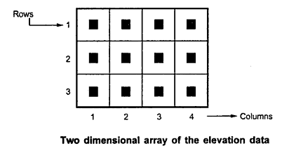
Each element in the array corresponds to a service area in the region whereas the actual content of the array element contains elevation information that is above the sea level. This is also known as “Digital elevation model”. It is also possible to use interpolation methods to find approximate heights (H) that are observed from radial point of view.
Using diagonal interpolation method terrain profile reconstruction can be done.
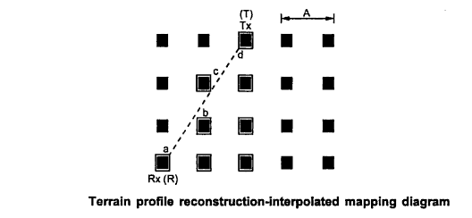
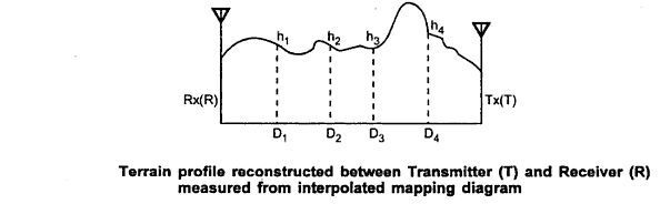
In the reconstructed terrain profile, the distance D1 to D4 are taken as,
D1 = R.a
D2 = R.b
D3 = R.c
D4 = R.d
also the diagram, shows the approximate heights h1 to h4 for each measuring point so that the elevation parameter will be made clear.
For Durking model measurements one of the important consideration is line of sight (LOS) path that is expected to be available between the radio transmitter and receiver (T-R) setup. For checking this a computer program develop should calculate the difference value in height denoted as dj. the height taken into account for finding dj is the height of the ground profile and height of the line that is joining the transmitter and receiver antennas for each and every point along the radial line.
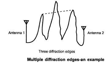
Among the four grades of the problem under non line of sight each are tested one by one for the particular terrain considered and the diffraction edge is detected by calculating the angles made between the line that join the transmitter (T) and the receiver (R ). This is done with reconstructed terrain profile. The maximum value of angle at a point is found at and labeled as (Di , hi). Also reverse process of calculating the angles is found and the line that joins the transmitter (T) and the receiver (R ) is measured. The maximum value of the angle is are calculated for every point on the terrain and the point is labeled as (Dj , 4j ). When the values Di is equal to Dj then the terrain profile considered is taken as a “single diffraction edge”. The losses if any, Path loss associated with the line joining T and R are also found.
In case the condition for the single diffraction edges does not exist then ‘test’ for two diffraction edges is carried out and so on. For the three diffraction edges case, generally the outer edges should contain one single diffraction edge available in between. The line between the two diffraction edges is measured for this iterative process. The process can be continued till multiple diffraction edges are offered. The Durkin’s method is popular since specific site-specific propagation nature is easily predicted. Also the path loss component (PL) and signal strength can also be measured
Okumura Model:
The Okumura model for Urban Areas is a Radio propagation model that was built using the data collected in the city of . The model is ideal for using in cities with many urban structures but not many tall blocking structures. The model served as a base for the Hata Model. Okumura model was built into three modes. The ones for urban, suburban and open areas. The model for urban areas was built first and used as the base for others.
Coverage:
Frequency = 200 MHz to 1900 MHz
Mathematical formulation:
The Okumura model is formally expressed as:
L = L(FSL) + A(MU) – H(MG) – H(BG) – Summation of K(Correction)
Where,
L = Median path loss; unit: Decibel(dB)
L(FSL) = The Free Space loss. unit: Decibel(dB)
A(MU) = Median attenuation. unit: Decibel(dB)
H(MG) = Mobile station antenna height gain factor.
H(BG) = Base station antenna height gain factor.
K(Correction) = Correction factor gain (such as type of environment, water surfaces, isolated obstacle etc.)
Points to note:
Okumura model does not provide a mean to measure the Free space loss. However, any standard method for calculating the free space loss can be used.
PCS Extension to Hata Model:
The European Co-operative for Scientific & Technical (EUROCOST) formed COST-231
- Extend Hatas model to 2GHz
L50 (urban)(dB) = 46.3 + 33.9logfc – 13.82 loghte – a(hre) + (44.9-6.55hte)logd + CM
fc = frequency from 1500MHz – 2 GHz
hte = 30m-200m
hre = 1m-10m
d = 1km-20km
Also read here
https://eevibes.com/computing/introduction-to-computing/ipv4-vs-ipv6/