The Frequent Pattern Growth (FP-Growth) algorithm is a highly efficient and popular algorithm for mining frequent itemsets from large transaction databases. It was proposed by Han, Pei, and Yin in 2000 as an improvement over the Apriori algorithm, primarily by avoiding the computationally expensive candidate generation step.
It’s widely used in areas like market basket analysis (e.g., “customers who buy bread and milk also tend to buy butter”), web usage mining, and bioinformatics, to discover hidden relationships and patterns in data.
Why FP-Growth? (Comparison to Apriori)
The traditional Apriori algorithm works by repeatedly scanning the database to generate candidate itemsets and then testing their support (frequency). This can be very inefficient, especially with large datasets or when dealing with long frequent itemsets, as it leads to:
- High computational cost: Due to numerous candidate generations.
- Multiple database scans: Which is time-consuming for large databases.
FP-Growth overcomes these limitations by using a divide-and-conquer strategy and a compact data structure called an FP-tree. It requires only two passes over the dataset.
Core Concepts:
- Itemset: A collection of one or more items (e.g., {Milk, Bread}).
- Support: The frequency of an itemset in the dataset (e.g., if {Milk, Bread} appears in 3 out of 10 transactions, its support is 3 or 30%).
- Minimum Support (Min_Sup): A user-defined threshold. Only itemsets with support greater than or equal to this threshold are considered “frequent.”
- Frequent Itemset: An itemset whose support is greater than or equal to the minimum support.
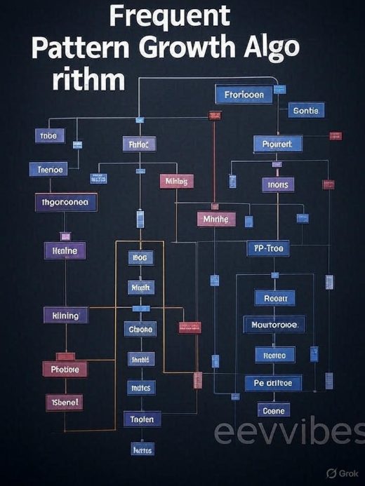
- FP-Tree (Frequent Pattern Tree): A highly compressed tree-like structure that stores the frequent itemsets in a hierarchical manner. It’s designed to be compact by sharing common prefixes among transactions.
- Conditional Pattern Base: For a given frequent item, it’s the set of prefix paths in the FP-tree that end with that item.
- Conditional FP-Tree: A smaller FP-tree constructed from a conditional pattern base.
How FP-Growth Algorithm Works (Two Main Steps):
Step 1: Construct the FP-Tree
This step involves two sub-passes over the original transaction database:
-
First Pass (Counting Frequencies):
- Scan the entire transaction database once.
- Count the frequency (support) of each individual item.
- Identify all items that meet the
Min_Supthreshold. These are the frequent 1-itemsets. - Sort these frequent items in descending order of their frequencies. This order is crucial for FP-tree compaction. Let’s call this the
F_list(or header table).
-
Second Pass (Building the Tree):
- Create the root node of the FP-tree, labeled “null”.
- Scan the transaction database a second time. For each transaction:
- Filter out the infrequent items from the transaction.
- Sort the remaining frequent items in the transaction according to the
F_list(descending order of global frequency). - Insert the sorted transaction into the FP-tree:
- Start from the root node.
- For each item in the sorted transaction, if the current node has a child corresponding to that item, traverse to that child and increment its count.
- If no such child exists, create a new child node for the item and link it from the current node. Increment its count to 1.
- Each newly created node also needs a node-link pointer that connects it to the next occurrence of the same item in the tree. These node-links are maintained in the header table, which contains each frequent item and a pointer to the first node in the FP-tree representing that item.
Example of FP-Tree Construction:
Let’s say we have the following transactions and Min_Sup = 2: