Histogram of Oriented Gradients (HOG) is a feature detection algorithm based on the image’s gradients. It is a classic approach for object detection in an image, e.g., a vehicle in the street, a pedestrian walking in the street, etc.

Examples of Histogram Oriented Gradient (HOG)

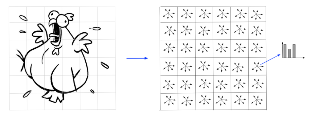
This algorithm operates based on the assumption that an image could often be described as a set (distribution) of gradients. In other words, we can convert an image into a set of gradients, such as Figure 1.

The above figure  sample figure on the left is binned into 6×6. (Right) each bin is presented with its gradient histogram (vectors are not real; they are just to show you how the image gets converted). Also, instead of presenting them on the X or Y axis, its vectors are presented among a central dot.

Another example is presented in Figure 2, in which the gradient of a real image is calculated and presented. Figures 2 presents the gradient in Sobel X and Sobel Y. In particular, the Sobel X filter detects edges with a change in intensity along the X-axis (horizontal edges).

It calculates the gradient by moving from left to right and emphasizes the differences in intensity between adjacent pixels in the left-right direction.

The Sobel Y filter detects edges with a change in intensity along the Y-axis (vertical edges). It calculates the gradient by moving from top to bottom and emphasizes the differences in intensity between adjacent pixels in the top- bottom direction.
The algorithm operation is straightforward. First, it divides the image into a grid of sub-images (cells), as you can see from Figure 1. Second, it calculates a histogram gradient of each cell. As a result, it will get something like the right side of Figure 1.

The set of histograms is used as a “feature vector” that describes the image or the object. Then, we fed these histograms into a classification algorithm and classified objects in our image.

One preliminary step is required at the beginning. Cells’ illumination invariance (e.g., lights and shadows) should be normalized or scaled, e.g., Min-Max scaling. Also, the authors of the HOG paper identified that L2 normalization performs better than other forms of normalization.

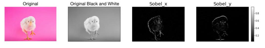
Figure above (Left) is a sample picture, which is then turned into black and white. Afterward, the X gradient and Y gradient of the image are calculated.
Since the HOG algorithm focuses on the gradient of a cell (local) rotation, scaling does not affect HOG values. Converting an image into gradients also causes the HIG feature descriptors to get compressed, which is very practical, especially on small devices, because image processing applications are usually resource-intensive.

Assuming the image has m x n size, the computational complexity of HOG is O(mn), which is linear. Scale Invariant Feature Transform (SIFT) is one of the most powerful image feature extraction algorithms, which can tolerate different types of noises, such as changes in illumination, viewpoints, and scaling.

When all images have the same size, orientation, and illumination, a simple corner detection such as HS or MSER works well. However, if images have different scales, viewpoints, rotations, or illuminations, SIFT can help.

Key Characteristics:

• Local Shape Information: HOG captures the direction and strength of edges, which represent the structure of objects.
• Robustness: Normalization makes it invariant to lighting and contrast changes.
• Applications: Widely used in pedestrian detection, face detection, and other object recognition tasks.

• Divide into 8×8 pixel cells → 8×16 cells total.
• Group into 2×2 cell blocks (16×16 pixels) with a stride of one cell → 7×15 blocks.
• Each block has 4 cells, each with a 9-bin histogram → 36 values per block.

• Total feature vector: 7x15x36=3780 features.

• Feed into an SVM for classification.

Example Image and MATLAB Code for HOG Implementation

% Read a more detailed image
img = imread(‘visionteam.jpg’); % You can also use ‘peppers.png’ or another detailed image

% Convert to grayscale if it’s RGB
if size(img,3) == 3
grayImg = rgb2gray(img);
else
grayImg = img;
end

% Display the grayscale image
figure;
imshow(grayImg);
title(‘Grayscale Image’);

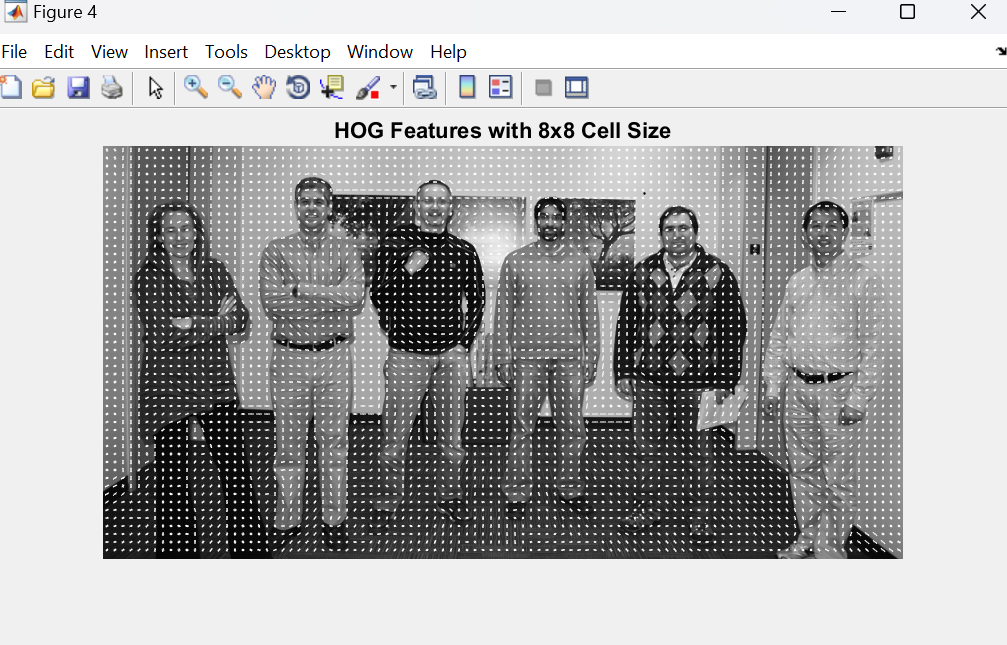
% Set a smaller cell size for finer detail
cellSize = [8 8];

% Extract HOG features and get the visualization data
[hogFeatures, visualization] = extractHOGFeatures(grayImg, ‘CellSize’, cellSize);

% Plot the HOG features over the image
figure;
imshow(grayImg); hold on;
plot(visualization);
title(‘HOG Features with 8×8 Cell Size’);

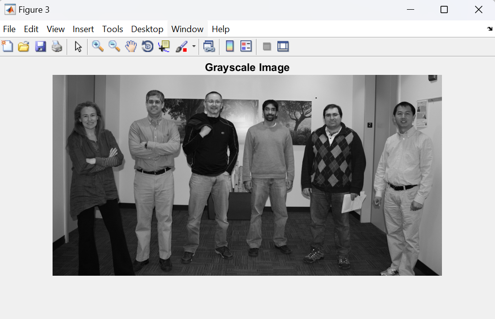
Image with HOG Features

Digit Classification Using HOG Features