Ridge Regression

Ridge Regression is a type of linear regression that adds a regularization term to the cost function to prevent overfitting, especially when predictors are highly correlated (multicollinearity). It modifies ordinary least squares by including an L2 penalty, which shrinks the regression coefficients toward zero without setting them exactly to zero.

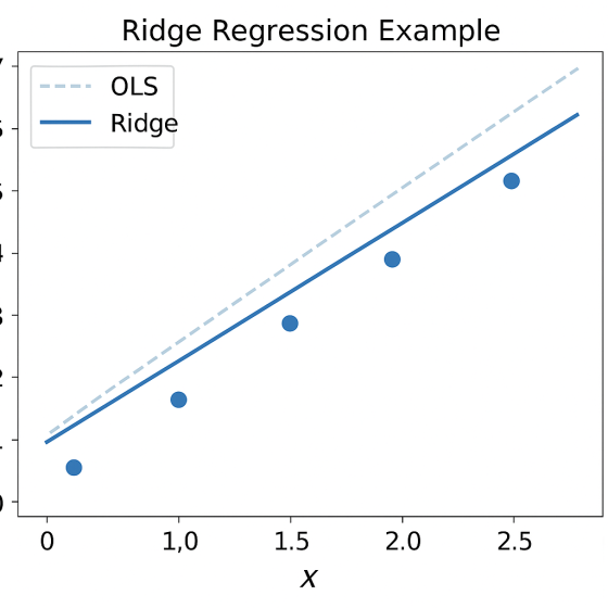
“Ridge regression addresses this problem by incorporating a regularization term into the ordinary least squares (OLS) objective function, which penalizes large coefficient values and thereby helps to reduce their variance.”

Ridge Regression’s Role in Combating Overfitting and Multicollinearity

Ridge Regression plays a critical role in combating overfitting and multicollinearity in linear regression models by introducing L2 regularization, which modifies the cost function to penalize large coefficients. Below, I explain how it addresses these issues, with a focus on its mechanisms, benefits, and practical implications.

Combating Overfitting

Overfitting occurs when a model fits the training data too closely, capturing noise rather than underlying patterns, leading to poor generalization on new data.

How Ridge Regression Works:

• Ridge Regression adds an L2 penalty term ($\lambda \sum_{j=1}^p \beta_j^2$) to the ordinary least squares (OLS) cost function: $$J(\beta) = \sum_{i=1}^n (y_i – \hat{y}_i)^2 + \lambda \sum_{j=1}^p \beta_j^2$$ where $\lambda$ controls the strength of the penalty.

• • This penalty shrinks the regression coefficients toward zero, reducing their magnitude, which limits the model complexity and prevents it from fitting noise in the training data.
• Why It Reduces Overfitting:
  • By shrinking coefficients, Ridge Regression reduces the model’s sensitivity to fit irrelevant or noisy predictors, lowering variance.
  • It enforces a smoother, more generalized model that performs better on unseen data.
  • The regularization parameter $\lambda$ balances the trade-off between fitting the data (bias) and model complexity (variance).
• Practical Impact:
  • Ridge is particularly effective when the training dataset is small or noisy, as these scenarios are prone to overfitting.
  • Cross-validation is used to tune $\lambda$, ensuring the model generalization without excessive bias.

2. Addressing Multicollinearity

Multicollinearity occurs when predictor variables are highly correlated, leading to unstable and inflated coefficient estimates in OLS regression, making interpretation unreliable.

• How Ridge Regression Helps:
  • In multicollinearity, correlated predictors lead to large, offsetting coefficients in OLS, inflating variance.
  • The L2 penalty in Ridge Regression constrains the coefficient magnitudes, stabilizing estimates by spreading the impact of correlated predictors more evenly.
  • Mathematically, Ridge modifies the normal equations by adding $\lambda I$ to the covariance matrix $X^T X$:$$\beta = (X^T X + \lambda I)^{-1} X^T y$$This ensures $X^T X + \lambda I$ is invertible, even when $X^T X$ is singular (common in multicollinearity).
  • Why It Works:
    • By shrinking coefficients, Ridge reduces the sensitivity to small changes in correlated predictors, producing more robust estimates.
    • It does not eliminate predictors (unlike Lasso), but dampens their influence, preserving all features while mitigating instability.
• Practical Impact:
  • Ridge is ideal for datasets with highly correlated predictors, such as in economics, genomics, or image processing.
  • It provides reliable coefficient estimates, even when the number of predictors approaches or exceeds the number of observations.

• Key Benefits of Ridge Regression

  • Overfitting: Reduces model variance, improving generalization to new data.
  • Multicollinearity: Stabilizes coefficient estimates, making the model more interpretable and robust.
  • High-Dimensional Data: Effective when predictors outnumber observations, as the L2 penalty ensures numerical stability.
  • Flexibility: The $\lambda$ parameter allows fine-tuning between OLS ($\lambda = 0$) and heavy regularization ($\lambda \gg 0$).

• 4. Limitations and Considerations

  • No Feature Selection: Ridge shrinks coefficients but never sets them to zero, so it’s not suitable if you need to select a subset of predictors (use Lasso or Elastic Net instead).
  • Feature Scaling Required: Since the L2 penalty depends on coefficient magnitude, predictors must be standardized (e.g., using StandardScaler).
  • Tuning $\lambda$: Requires computational effort, typically via cross-validation, to find the optimal regularization strength.
  • Bias Introduction: Shrinkage increases bias, which may reduce accuracy if the true model requires large coefficients.

5. Practical Implementation

Here’s how to implement Ridge Regression in Python using sklearn to address overfitting and multicollinearity:

import numpy as np
from sklearn.linear_model import Ridge
from sklearn.preprocessing import StandardScaler
from sklearn.pipeline import make_pipeline
from sklearn.model_selection import cross_val_score

# Generate sample data
np.random.seed(42)
X_train = np.random.rand(100, 3) # 100 samples, 3 features
y_train = np.random.rand(100) # 100 target values
X_test = np.random.rand(20, 3) # 20 test samples

# Create a pipeline to scale features and apply Ridge
ridge = make_pipeline(StandardScaler(), Ridge(alpha=1.0)) # alpha = λ

# Fit model
ridge.fit(X_train, y_train)

# Predict
predictions = ridge.predict(X_test)

# Tune λ using cross-validation
from sklearn.linear_model import RidgeCV
ridge_cv = make_pipeline(StandardScaler(), RidgeCV(alphas=[0.1, 1.0, 10.0]))
ridge_cv.fit(X_train, y_train)
print(“Optimal λ:”, ridge_cv.named_steps[‘ridgecv’].alpha_)

8. Visualizing the Effect of Ridge Regression

To illustrate how Ridge Regression shrinks coefficients, consider plotting coefficient magnitudes across different $\lambda$ values. Below is a chart showing how coefficients change as $\lambda$ increases:

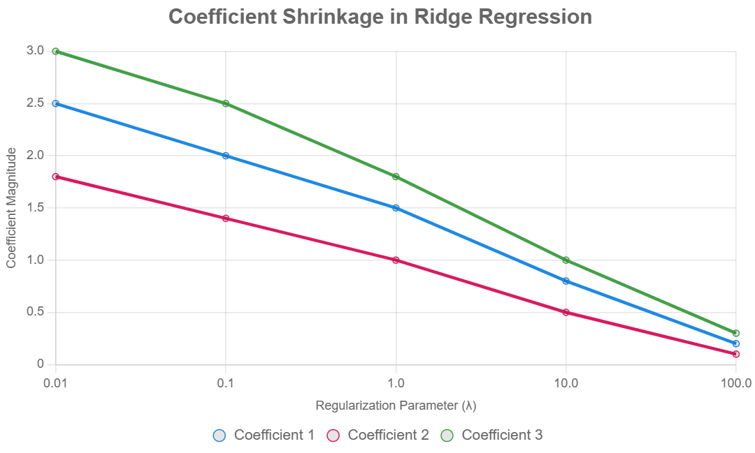
This chart shows that as $\lambda$ increases, coefficient magnitudes decrease, reducing overfitting and stabilizing estimates for correlated predictors.

Bias-Variance Tradeoff in Ridge Regression

Ridge Regression effectively addresses the bias-variance tradeoff by introducing a regularization term into the ordinary least squares (OLS) loss function. This regularization term penalizes large coefficients, which reduces the model’s variance at the cost of introducing a small amount of bias.

In traditional linear regression, especially when dealing with multicollinearity or high-dimensional data, the model may overfit the training data, resulting in low bias but high variance.

Ridge Regression mitigates this by shrinking the coefficients towards zero, thus simplifying the model and making it less sensitive to fluctuations in the training data.

As the regularization parameter λ increases, the model becomes more biased but gains stability, reducing variance and improving its ability to generalize to unseen data. Therefore, Ridge Regression finds a balance between underfitting and overfitting by managing this tradeoff, often leading to better overall predictive performance.

Conclusion

Ridge Regression is a powerful tool for addressing overfitting and multicollinearity by introducing L2 regularization. It shrinks coefficients to reduce model variance and stabilize estimates, making it ideal for datasets with correlated predictors or high-dimensional settings. While it doesn’t perform feature selection, its ability to handle multicollinearity and improve generalization makes it a go-to method in many applications. Proper tuning of $\lambda$ and feature scaling are key to maximizing its effectiveness.