Introduction
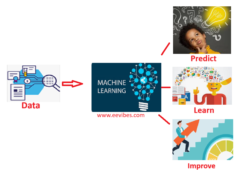
Machine learning is a transformative branch of artificial intelligence that empowers computers to learn from data and make decisions without explicit programming. At its core, machine learning involves developing algorithms that can recognize patterns, predict outcomes, and adapt to new information through iterative processes.
This paradigm represents a significant shift from traditional programming approaches, where rules and logic are manually defined by developers.
Supervised and Unsupervised Learning
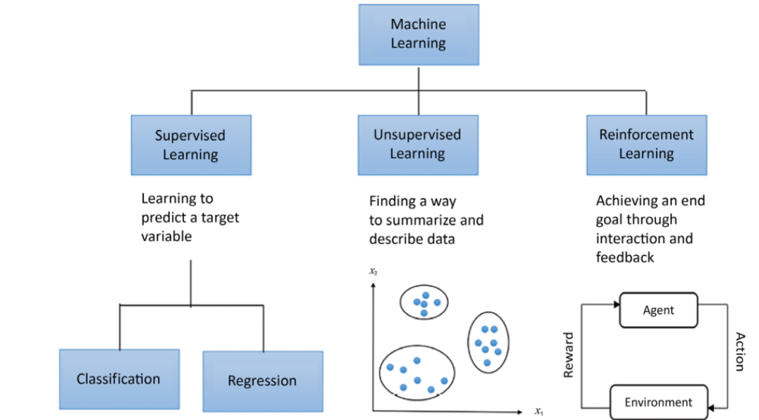
Machine learning is broadly categorized into three types:
- supervised learning,
- unsupervised learning,
- and reinforcement learning.
Supervised Learning
Supervised learning involves training a model on a labeled dataset, where the algorithm learns to map inputs to known outputs. This approach is utilized in tasks such as classification, where data is categorized into predefined classes, and regression, where continuous outcomes are predicted based on input features.
For instance, supervised learning models can predict housing prices based on historical data or classify emails as spam or not spam.
Unsupervised Learning
Unsupervised learning deals with unlabeled data and aims to uncover hidden structures or patterns within the data. This type of learning is applied in clustering, where data points are grouped based on similarities, and dimensionality reduction, where the number of features is reduced while preserving essential information.
Unsupervised learning is instrumental in identifying customer segments or simplifying complex datasets.

Reinforcement Learning
Reinforcement learning is a technique where an agent learns to make decisions by interacting with an environment and receiving feedback in the form of rewards or penalties. This approach is commonly used in scenarios that involve sequential decision- making, such as game playing, robotics, and autonomous driving. The agent aims to maximize cumulative rewards over time by learning optimal strategies through trial and error.
Fundamental Elements of Machine Learning
The foundational elements of machine learning include:
- algorithms,
- data, and
- evaluation metrics
Algorithms are the mathematical models and computational procedures used to process data and generate predictions. Common algorithms include decision trees, support vector machines, neural networks, and ensemble methods.
The quality and quantity of data significantly impact the performance of machine learning models; hence, data preprocessing and feature engineering are critical steps in ensuring model accuracy.
Evaluation metrics, such as accuracy, precision, recall, and F1-score, assess the performance of models and guide improvements.
Machine learning has seen rapid advancements due to the increasing availability of data, powerful computing resources, and sophisticated algorithms.
Its applications span various domains, including healthcare, finance, marketing, and autonomous systems. By leveraging machine learning, organizations can uncover insights from complex datasets, automate decision-making processes, and drive innovation in numerous fields.
The continuous evolution of machine learning techniques and technologies promises to further enhance its capabilities and impact on society.
Decision Trees and Random Forests
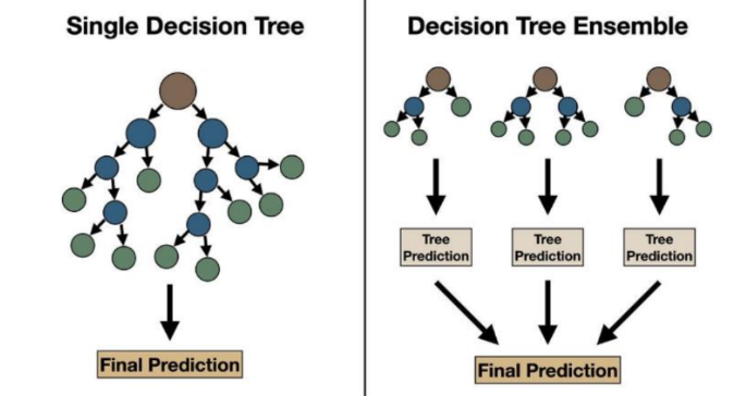
Decision trees and random forests are fundamental machine learning algorithms used for both classification and regression tasks. These methods provide intuitive, interpretable models and are widely employed due to their effectiveness in handling various types of data.
Decision Trees are hierarchical models that recursively split the data into subsets based on feature values. The process begins with the entire dataset and progressively divides it into smaller groups based on criteria that maximize the separation of the target variable.
Each internal node in the tree represents a decision based on a feature, while each leaf node corresponds to a predicted outcome or class label.
The splits are determined by metrics such as Gini impurity, entropy, or mean squared error, depending on whether the task is classification or regression. Decision trees are prized for their interpretability, as they visually represent the decision-making process. However, they are prone to overfitting, especially with complex datasets that lead to excessively deep trees.
Random Forests
Random Forests address the limitations of decision trees by constructing an ensemble of trees, each trained on a random subset of the data and features. This technique, known as bootstrap aggregating or bagging, improves model robustness and accuracy by combining the predictions of multiple decision trees.
Each tree in a random forest votes for a class label or regression value, and the final prediction is determined by majority voting (for classification) or averaging (for regression).
Random forests mitigate the overfitting issue common in single decision trees, as the averaging of multiple trees reduces variance and improves generalization.
Additionally, random forests provide measures of feature importance, offering insights into which features contribute most significantly to predictions.
Both decision trees and random forests are versatile tools that can handle numerical and categorical data and are capable of modeling complex relationships.
Their ability to deal with high-dimensional data and provide interpretable results makes them valuable for a wide range of applications, including finance, healthcare, and marketing.
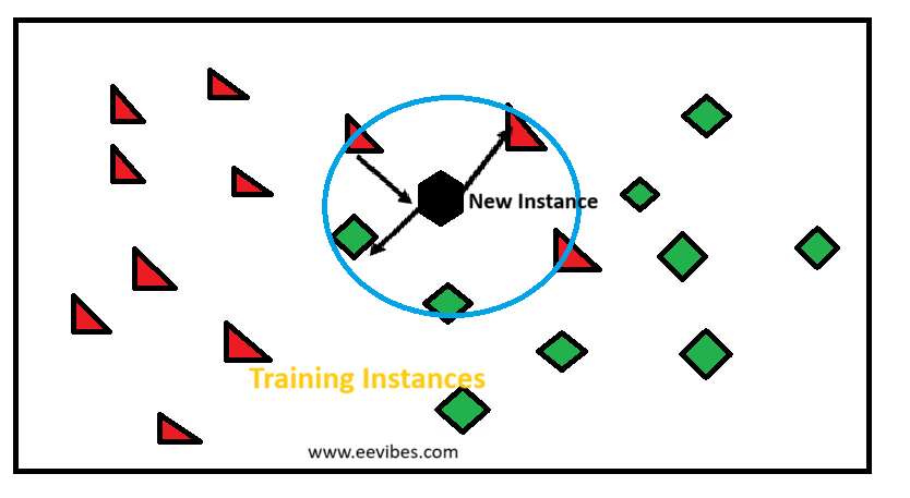
K-Nearest Neighbors (KNN)
K-Nearest Neighbors (KNN) is a widely used algorithm in machine learning for classification and regression tasks. It is a type of instance-based learning or lazy learning, where the model learns from the training data at the time of prediction rather than through an explicit training phase.
The simplicity and effectiveness of KNN make it a popular choice for various applications. The core concept behind KNN is to classify or predict the output for a given data point based on the majority class or average of its nearest neighbors in the feature space.
In classification tasks, the algorithm assigns a class label to a data point based on the most frequent class among its ‘k’ closest neighbors.
For regression tasks, KNN predicts the value by averaging the values of its ‘k’ nearest neighbors. The process begins with calculating the distance between the data point of interest and all other points in the training dataset.
Common distance metrics include Euclidean distance, Manhattan distance, and Minkowski distance. Once the distances are computed, the algorithm identifies the ‘k’ closest data points.
The parameter ‘k’ is a critical hyperparameter that affects the algorithm’s performance; choosing an appropriate value for ‘k’ is essential to avoid overfitting or underfitting.
In classification, the majority class among these ‘k’ neighbors is assigned to the data point, whereas in regression, the prediction is made by averaging the target values of the ‘k’ nearest neighbors. The choice of ‘k’ influences the decision boundary and can affect the model’s accuracy.
A smaller ‘k’ value might lead to a model that is sensitive to noise in the data, while a larger ‘k’ can smooth out the decision boundary but may also blur class distinctions.
KNN is highly intuitive and easy to implement, with its primary advantage being that it requires no explicit training phase. Instead, it stores the entire training dataset and performs computations only when a prediction is needed. This characteristic, however, means that KNN can become computationally expensive, especially with large datasets, as it requires distance calculations for every query point.
The algorithm is also sensitive to the scale of the data; features with larger scales can disproportionately influence the distance calculations. Therefore, feature scaling or normalization is often recommended to ensure that all features contribute equally to the distance metric.
Despite its simplicity, KNN performs well in many scenarios, particularly when the decision boundaries are not linear. Its effectiveness depends on the choice of ‘k’, the distance metric, and the quality of the input features. In practice, KNN is often used as a baseline model or in combination with other algorithms to improve performance in classification and regression tasks.
Overall, K-Nearest Neighbors is a versatile algorithm that leverages proximity in feature space to make predictions, offering a straightforward yet powerful approach to various machine learning problems.
Dimensionality Reduction: PCA
Dimensionality reduction is a critical technique in data analysis, aimed at reducing the number of features or variables in a dataset while retaining its essential structure and information. Principal Component Analysis (PCA) is one of the most widely used methods for dimensionality reduction and plays a significant role in simplifying data, improving computational efficiency, and enhancing visualization.
PCA operates by transforming the original features into a new set of orthogonal axes known as principal components. These components are derived from the eigenvectors of the covariance matrix of the data, and they capture the directions of maximum variance in the dataset.
The principal components are ranked according to the amount of variance they explain, with the first component capturing the highest variance, the second component capturing the next highest variance, and so on.
The process of PCA begins with standardizing the data, particularly when the features have different units or scales, to ensure that each feature contributes equally to the analysis. The standardized data is then used to compute the covariance matrix, which measures the relationships between pairs of features.
Eigenvalue decomposition of this matrix yields the eigenvectors and eigenvalues. The eigenvectors, or principal components, define the new feature space, while the eigenvalues indicate the amount of variance captured by each component.
Also read here: