What is a Dipole Antenna?

What is the Dipole Antenna? An antenna is used for transmitting or receiving radio frequency energy has a center-fed driving element. The simplest and most common type of antenna in radio and telecommunications is a dipole antenna, sometimes known as a doublet.

Usually, a dipole antenna is made up of two identical conducting components, like metal wires or rods. Between the two parts of the antenna, the driving current from the transmitter is applied, or for receiving antennas, the output signal to the receiver is taken. One of the conductors is linked to each side of the feed line going to the transmitter or receiver.

The “rabbit ears” television antenna used on broadcast television sets is a typical illustration of a dipole.

Construction of a Dipole Antenna

Heinrich Hertz, a German physicist, created the dipole antenna in 1886.

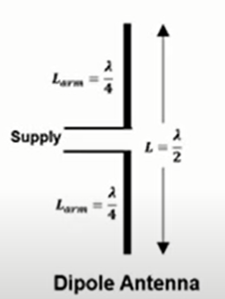
It is made up of a metal bar that is half as long as the longest wavelength the antenna is intended to produce. The two halves of this metallic bar are separated down the middle, with an insulator separating them. A coaxial wire is attached to each rod’s end nearest to the antenna’s center. Dipole antennas receive radio frequency voltages at their center, in-between the two wires.

Working of a Dipole Antenna

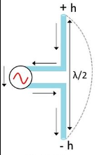
When the radio frequency voltage source is applied between the both conducting rods in the antenna, voltage and current are flowed throughout the whole structure. And, electromagnetic signals are produced whose radiance is flowed to the exterior of the antenna. The minimum voltage and maximum current is observed right at the center of the antenna. At the ends, it will be reciprocating. This is how the current is distributed in the dipole antenna.

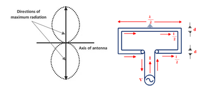
The radiation pattern is really vital in the working of dipole antenna as it depicts the flow of EM waves. The emission of energy in the space is observed through the radiation pattern. The pattern is vertical to the axis of antenna.

Dipole antenna’s purpose is to convert the electrical signals into the radio frequency electromagnetic signals. And afterwards, the emission is observed at the transmitting end of the antenna. And at the receiving end, the signals are reciprocally inverted.

The dipole antennas are really vital for telecommunication and transmission purposes as they are highly efficient in terms of gain and efficiency levels.

Types of Dipole Antenna

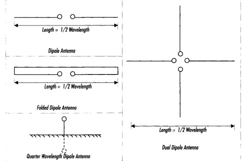
Dipoles are in four types:

• Half-wavelength dipole
• Quarter-wavelength dipole
• Dual dipole antenna
• Folded dipole

1. Half-wavelength dipole:

This antenna’s overall length is equal to half of the wavelength that relates to the desired frequency. The power transfer between the tag and reader is optimized.

2. Quarter-wavelength dipole:

The overall length of this antenna is equivalent to one-fourth of the wavelength for the targeted frequency. The dipole is completed using the reflecting ground plane, which is also used to project an image of the antenna.

3. Dual dipole antenna:

A dual dipole antenna has two dipoles as its name indicates. The precision of a tag’s direction is diminished because it reaches a greater area.

4. Folded dipole antenna:

Each electric conductor in this antenna is half as long as the wavelength corresponding to the frequency to be used, and it is made up of two or more straight electric conductors linked in parallel.

HFSS (High Frequency Simulation Software):

HFSS is a simulating software in which complex structures can be modelled with much more accuracy. This applies the new technologies within the same local directory. The parameters plotting can be visually interpreted through this software. It is the most reliable software for the electromagnetic depiction of the waves.

VARIOUS PARAMETERS OF THE DIPOLE ANTENNA:

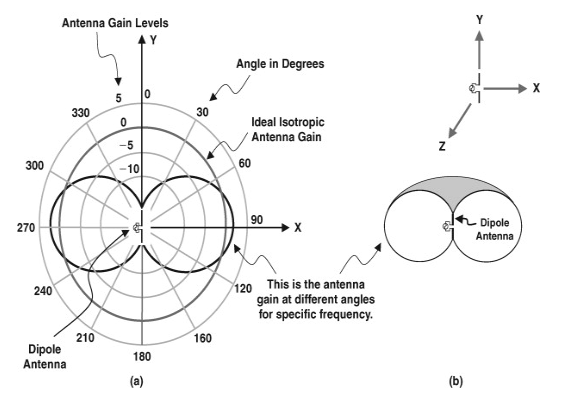
 Radiation Pattern:

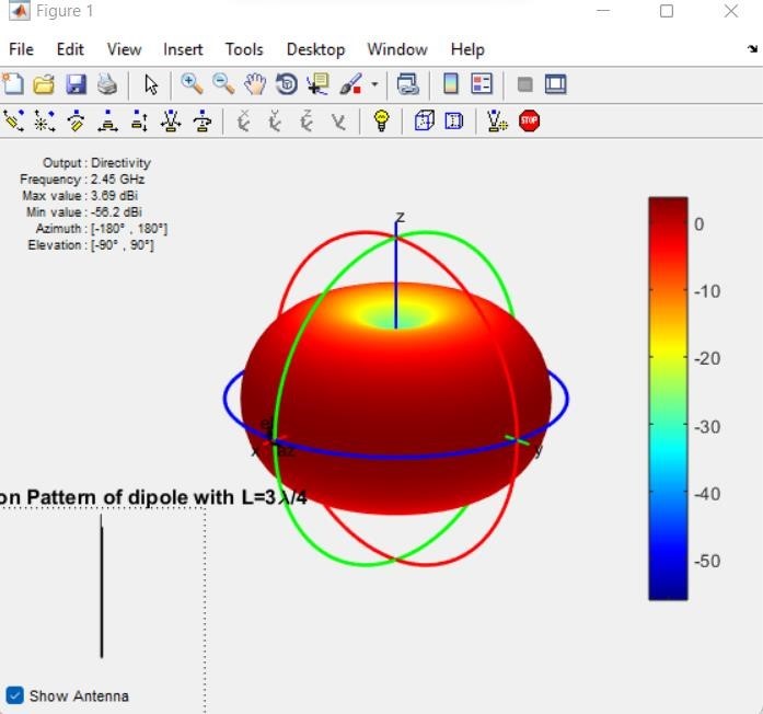
The graphic demonstration of radiations is termed as the radiation pattern. In X-Z coordinates, the radiation pattern resembles that of an ideal isotropic antenna. The donut-shaped radiation pattern is the term used to describe the three-dimensional radiation pattern of a dipole. Linear polarization is present. The pattern is vertical to the axis of the dipole antenna.

Maximum radiation is observed at the horizontal axis if the dipole antenna is placed vertically. And, if antenna is placed horizontally, the radiation pattern will be at peak and null at the vertical axis.

Impedance of the Antenna

The impedance optimization of the dipole antenna is demonstrated. It can alter when it is passed through the length of the antenna. If the dipole antenna input is small, impedance would be of capacitive nature. If the input is large, then the impedance will decrease. A resistor can roughly simulate a perfect dipole antenna that isn’t near any conducting or dielectric materials. The choice of dielectric material and distance from a ground might alter the antenna impedance if a dipole is installed on a PCB. By altering the wire’s length or shape, the antenna impedance can be adjusted.

The impedance of the feed point is dependent on the length and the feed position of the dipole antenna.

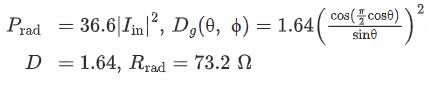
The input impedance constitutes of two parts imaginary and the real.  The plotting is demonstrated between the impedance and the frequency. The 73 ohms is real component impedance ( of the resonance frequency. So, the imaginary component is 42.5 ohms. These components formulas are given below

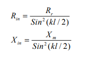
Where, assumption is brought that length (l) is greater than the diameter (a) of the dipole antenna.  is the radiation resistance at .

is the real component of input radiation resistance, whereas,  is the imaginary component of input radiation resistance.

The resistance of the radiation is basically the input impedance of the antenna as  for  is at the terminals of the input component. The imaginary component is linked with the length of the antenna. Hence, the total input impedance for the half wavelength is equal to =73+j42.5 ohms.

Resistance of the radiation at the input terminals is boundless.

Hence, verification can be performed and the multiple of wavelength is the length given as,

L=n λ, where n is the positive integer

Field Regions of Dipole Antenna

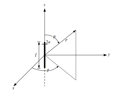
Cutting the dipole antenna into small parts and then adding up the separate fields can be used to determine the radiation fields if it is not electrically tiny and the current distribution is understood. Each component can be imitated by a small dipole with a distinct excitation current and location.

An Arbitrary-Length Linear Dipole Antenna might be considered to be composed of numerous tiny dipole “slices.” The overall field can be determined by adding the fields produced by each tiny dipole slice’s current I(z), length z, and placement at a distance z from the midpoint.

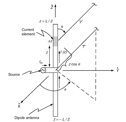
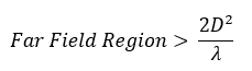
Far Field Region

The region which is farther away from the antenna is termed as the far field region. Equations described below can be used to express the elemental field ∆E produced by a current element of length z, situated at a distance z from the center, with a current.

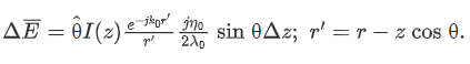
Letting z<< r in the far-field, then the equation can be made simpler by estimating the r′ in the r as the denominator,

By integrating the equation with respect to z, from z = L/2 to z = +L/2, the total field can be found,

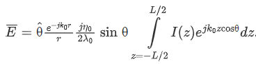
The far-field of the entire antenna can be calculated using the mentioned equation if the current distribution I(z) is known or can be roughly approximated by a known function. One would anticipate a standing wave pattern in the current distribution, with zero current at the line’s ends (z = L/2) and   in the middle. This behavior resembles the current distribution along a transmission line that is open-circuited and has a propagation constant of .

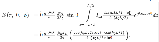
We can get a close form formula for the far-field distribution by using the current distribution of equations in the total field equation and then integrating over z,

The basic mathematical formulas explaining the operation of antennas and the radiation of electromagnetic energy are found in Maxwell’s equations. They assert that alternating magnetic fields must exist if there is an alternating electric field, and vice versa. Depending on the medium through which the electromagnetic field is propagating, each has a different relative magnitude.

Here, the field regions dominate the Electromagnetic field region. The formula is given below,

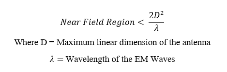
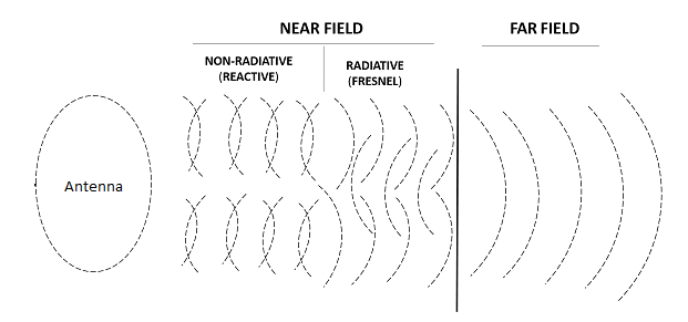
Nearer Field Region

The field region which is in the neighborhood of antenna is termed as the nearer field region. The formula for the nearer field region is given below, in which D is the maximum linear dimension of the antenna and  is the wavelength of the electromagnetic waves. The overlapping of the field lines is observed.

Non- Radiative near field have perpendicularly out of phase and orthogonal electromagnetic field.

Radiative near field is the region among the non-radiative near field and the far field. Here, the transition happens.

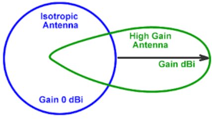
What is the Directivity of the Dipole Antenna?

The directivity of the dipole antenna is a vital parameter which calculates the degree to which the emission of radiation pattern is condensed in one direction. The ratio of both intensity of radiation in a specific mentioned direction and the intensity of radiation dispersed in all the directions. Thus, the directivity of an isotropic antenna radiator is termed as 1 or either 0 relative decibels.

The directivity of antenna is given by the following formula,

Directivity (D)= Gain/Efficiency

It can be further derived from these equations as,

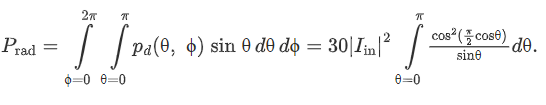
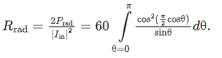
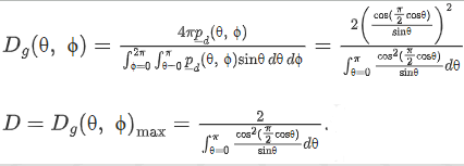
The θ integral that identically appears in the above equations may be computed numerically and has an approximate value of 1.22.

Using this value, the antenna parameters can be approximated as follows:

We can note that the directivity D of a half-wave dipole (= 1 .64) is not primarily different from that of a small dipole (= 1.5).

Gain of the Dipole Antenna:

 

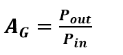
Gain is the measurement of an antenna’s potential to radiate EM waves in a particular fixed direction. It is the ratio between the two values that of the energy radiated at the locus where radiation is maximum, And the energy radiated at the fixed locus in reference of an antenna,

The reference antenna is known as an isotropic antenna because it radiates power systematically in all the directions. Hence, the radiated power of the reference antenna can be considered as equal to that of the input power, with the assumption that there are no losses. The new equation is formed as,

Antenna gain is expressed in decibels,

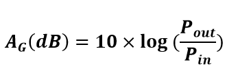
The total output power which is transmitted is not larger than the input total power. The output power in a specified direction is greater than the reference power in the same specified direction. It means that the antenna’s working principle is not that of an amplifier.

 

A transmission line is used in receiving the power from the source prior to the power transmission. That’s why impedance is also important as it is the characteristic of the transmission line.

The dipole antennas are mostly in cylindrical shape and they have limited power gain because of their extensive radiations. The dipole antenna is not categorized in directive antennas, as its power is radiated 360 degrees all over the antenna. It is the major reason of the limited power gain.  A dipole antenna is required in the transportability devices, as there is no access point available for the next connections. If the device track down the access point at the north of its position, the radiations will continue to emerge throughout the all directions. It will create noise and interrupt other AP’s in the region of the same channels.

Efficiency Level of Dipole Antenna

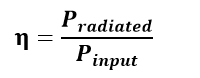
The efficiency of an antenna is its most significant element. Efficiency is referred to as the ratio of a dipole’s input power to its transmitted power. High efficiency dipole antennas have substantial transmitted power at the receiver, but low efficiency dipole antennas have high internal power losses.

A dipole antenna as a transmitter and receiver needs to be effective. The potential power from every directing angle together determines the dipole antenna’s effectiveness. The following formula can be used to calculate efficiency:

 

For the space-wave efficiency (η), the expression is,

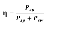
Where,  is the surface-wave power  and   is the space-wave power.

Although efficiency is measured in percentages, it can also be measured in decibels (dBi) for dipole antennas. In reality, there are losses that prevent us from having a 100% efficient antenna. These losses are,

• Conductive losses
• Dielectric losses
• Impedance mismatch losses

Half wave-length dipole antenna is the most effective antenna in terms of efficiency.

 

• Dipole Antenna’s Frequency Parameter:

There are several ranges of frequency bands of radio waves in a spectrum for the development of the dipole antenna. We can build variety of dipoles of varying frequencies starting from high to ultra-high. As the relationship indicates that the radio wave’s frequency and wavelength are inversely correlated. As a result, we can see that the dipole antenna’s length and frequency are inversely related. The wavelength can be determined using the dipole’s frequency.

Designated frequency of Dipole Antenna,

f=2.4GHz

As,

$$
\begin{gathered}
\lambda=\frac{\boldsymbol{c}}{\boldsymbol{f}} \\
\lambda=\frac{3 \times 10^8 \mathrm{~m} / \mathrm{sec}}{2.4 \times 10^9 \mathrm{~Hz}} \\
\lambda=0.125 \mathrm{~m} \\
\boldsymbol{\lambda}=\mathbf{1 2 5} \mathbf{~ m m}
\end{gathered}
$$
Length of the dipole (L),
$$
\begin{gathered}
L=\frac{\lambda}{2} \\
L=\frac{125 \mathrm{~mm}}{2} \\
\boldsymbol{L}=62.5 \mathrm{~mm}
\end{gathered}
$$
Arm Length $\left(L_{a r m}\right)$,
$$
\begin{gathered}
L_{\text {arm }}=\frac{\mathrm{L}}{2} \\
L_{\text {arm }}=\frac{62.5 \mathrm{~mm}}{2} \\
\boldsymbol{L}_{\text {arm }}=\mathbf{3 1 . 2 5} \mathbf{~ m m}
\end{gathered}
$$

The hardware-software facility for vertical-incidence ionosphere sounding, which was created on the basis of the R-017 and a personal computer, was used to measure the ionosphere parameters.

Features of Hardware-Software Facility for Vertical-Incidence Ionosphere Sounding

The facility has some of the following features:

• 50 Hz sound pulse repetition rate and a transmitter pulse power of 2 kW.
• The broadband delta-type antenna was utilized to send the impulse signal in the vertical-incidence sounding mode, with the primary lobe of the beam being 60 degrees wide. As receiving antennas, half-wave dipoles operating at 6 MHz—the working range’s mean frequency—were employed. When operated at fixed frequency, the facility provided a Doppler spectrum of the ionosphere-reflected radio signal, as well as making it possible to calculate the weighted mean frequency Doppler shift. Twenty seconds was chosen as the spectral analysis interval, resulting in a frequency resolution of 0.05 Hz. The frequency band 6 Hz was used for the spectral analysis.
• With a signal-to-noise ratio of at least 10, observations lasting from 15 minutes to several hours were made. Working frequencies in the range of 2-4 mHz were utilized in the experiment, and the signal reflected from the ionosphere was picked up. The induction magnetometer was used to continuously capture geomagnetic pulsations in the frequency range of 0.5-0.005 Hz and in the dynamic range of 0.01-100.

Steps of Designing the Dipole Antenna

Step 1- Initiating the project directory file

 

• Firstly, initiate by running the HFSS Software.
• Then, create the new project directory file from the project manager window at the top left corner of the screen. Name the file “dipole123” and press save from the sub window.

• Insert the HFSS design by right clicking the project file being made in order to set the configurations.

 

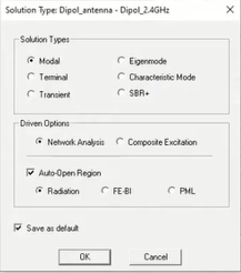
Step 2- Defining the variables

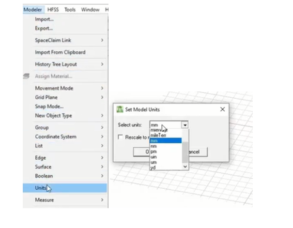
Click the solution type and driven modal from the HFSS window

• Set the units to be “mm” and open the 3D modelling window.

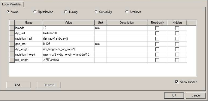
• Variables holds importance in HFSS project.

1. With the help of variables the length, height and width are maintained through specified ratios.
2. The designing of the project is optimized according to the need of the user.
3. The dimensions can be altered easily in a single window.

So, from the HFSS in the top menu, choose the design properties.

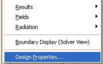
• A table will open up, Add the required variables with the unit of mm.

Step 3- Creating the Model

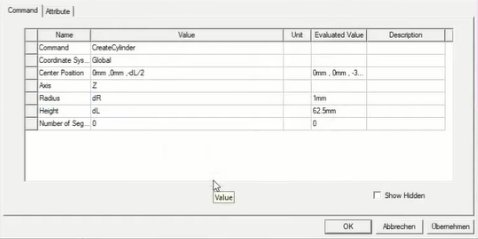
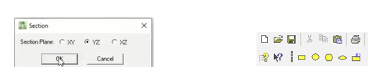
• From the 3D modeler toolbar at the top (as all the geometric structures are specified there), click the cylinder and draw it on the plane.

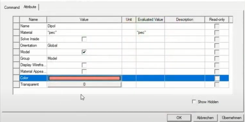
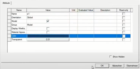
• Now, for the structure size, name the object and select “pec (perfect electric conductor)”

And then press OK. It will help in creating the ideal conditions for the antenna.

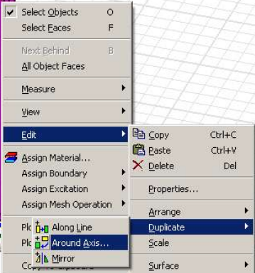
In the command tab of the same window,

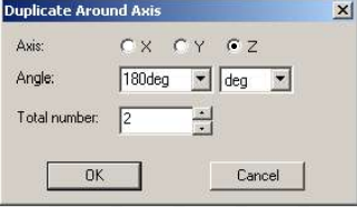
• As, we are dealing with dipole, we need symmetry in the structures. Press edit and then duplicate “around the axis”.

• A mirror image is created by setting the angle 180 degree.

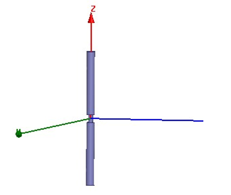
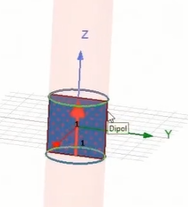
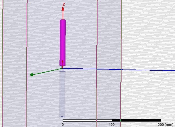
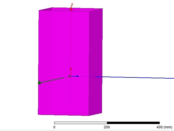
A dipole structure is demonstrated,

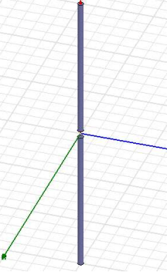
A space slot has been placed at the origin in order to place the source.

Step-4 Creating the port

• A lumped gap source is created in order to produce excitation to the dipole.

Select the plane and draw a rectangle in the modelling area.

• Set the parameters in the attribute and command tab of the 3D modeler.

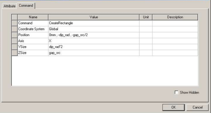
• The gap source is comparatively small than the dipole structure in order to emphasize the focus on the dipole and to lessen the effects on the structure.

 

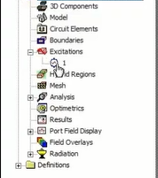
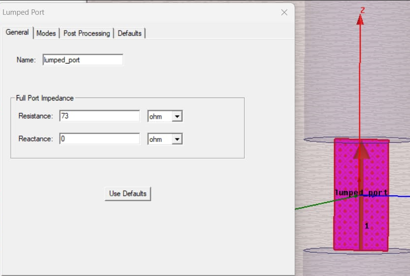
• To provide excitation, go to the excitation in the explorer and assign the “lumped port”.

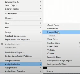
• Name the port and set the default values.
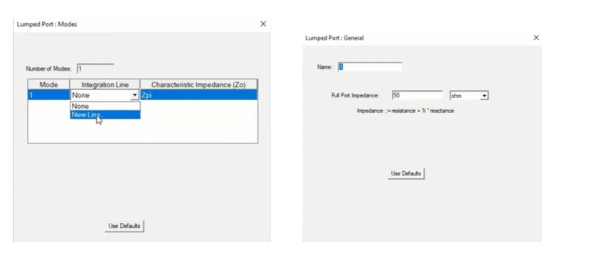• For the completion of the port excitation, Position the cursor according to your feasibility and define the origin of the field vector by left clicking at the bottom center. Then again by left clicking and taking the cursor to the top center, we can conclude the field vector.

Excitation is provided to the lumped source,

Step5- The Radiation Boundary

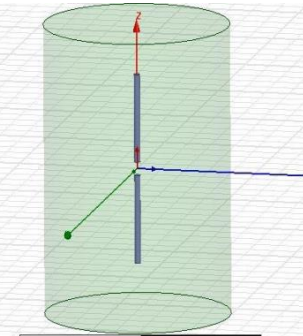
• To attain extraction of far field particulars from the dipole structure, we introduced the radiation boundary. For this, a cylindrical boundary is interpreted by drawing a cylinder with a distance of on the model area.

• Set the parameters in the attribute and command tab of the 3D modeller.

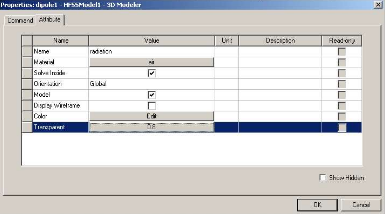
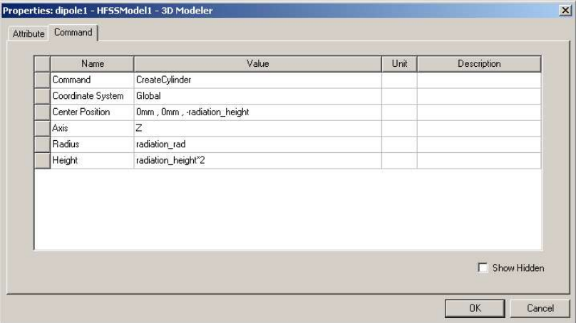
With the radiation boundaries, the structure is demonstrated as,

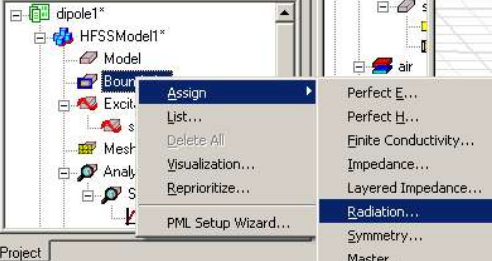
Pick all the faces from the 3D toolbar window

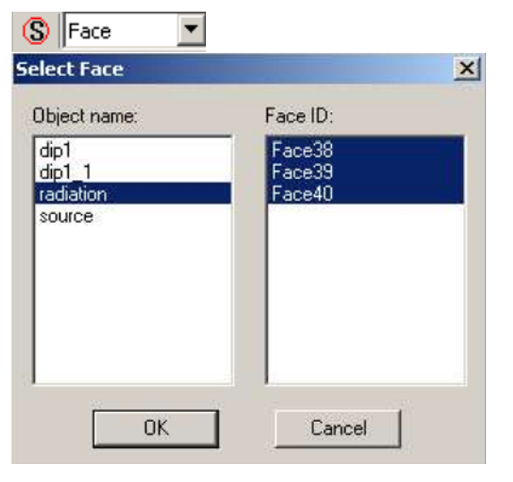
• Choose the boundary from the explorer window and then select assign and “radiation”.

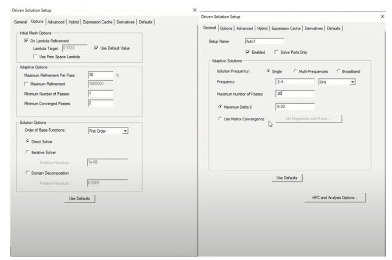
Step -6 Setting up the Solution

We’ll calculate all the parameters required like, frequency, radiation pattern, field regions, directivity, gain, impedance and efficiency. As, HFSS display all the user-desired data.

• Choose analysis and then add the solution setup from the explorer window.

• Set the parameters to default and then press OK.

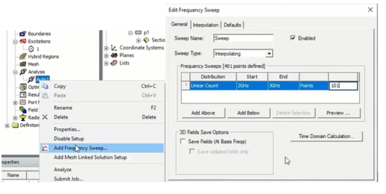
Step7-Frequency Response of the Dipole Structure

 

• In order to outlook the frequency response of the dipole structure, define a frequency sweep by adding sweep from the setup at the analysis bar.

Step 8-Analysis of the Dipole structure

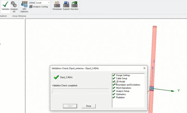
• Firstly, for the verification of the project, press the “tick sign” in the 3D bar menu.

One can verify the correctness of the structure drawn. Specifically,

• 3D model
• Boundaries and Excitations
• Mesh Operations
• Analysis Setup
• Optometric
• Radiation
• The tick sign will be displayed in front of the parameters to show that these are correct.

The analysis will take some time.

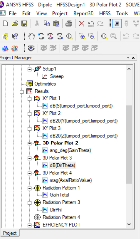
Step 9- Generating Reports

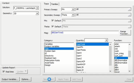
• We can analyze the frequency and the radiation format by generating the reports from the HFSS in the top menu, then pick results and “create reports”.

• And, press analyze all.

• Choose “new reports” by adding all the traces after highlighting all the parameters, this way it will load in the trace window.

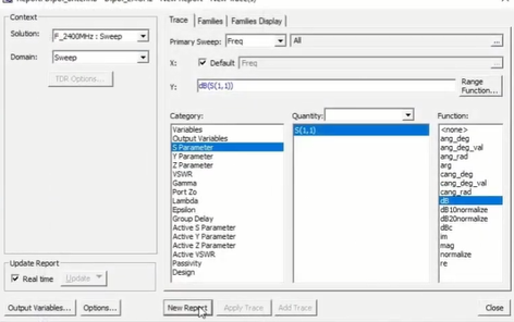
• Press “Done”.

All the output plots will be exhibited.

• The resistance can be calculated directly from the graph plot by marking the point where the imaginary part passes zero. Here, impedance can be calculated at the specified resonant frequency. The resistance would be,

• Then, zoom in at the marked point to analyze.

• And, trace the zero point by choosing the “Add marker” from the plot menu.

• Mark the point as near as possible to the zero across the imaginary line by left clicking.
• Then press “Fit all” by right clicking the plot menu.

• Repeat the procedure for the real part at the specified frequency.
• Then, analyze the S- plot with the same procedure of trace. Then press “done”.
• Click analysis and then “revert to initial mesh” to feed the memory. By this we can have re analyzation of the structure.

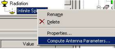
• For the far field calculations, we had to insert the far field setup then the “infinite sphere”.

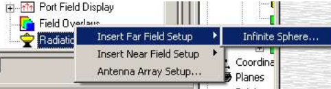
• Set the default parameters and then press infinite sphere1 then “compute antenna parameters” from the project menu.

• The far field plot will be attained. Generate the report and perform some modifications.

The result will be displayed and all the plotting can be visualized.

Simulations of the Dipole Antenna 

With the Boundaries:

In the Vacuum:

SIMULATION OF THE PARAMETERS OF THE DIPOLE ANTENNA:

• The Efficiency Plot of the Dipole Antenna

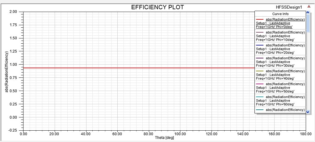
• The S Parameters of the Dipole Antenna

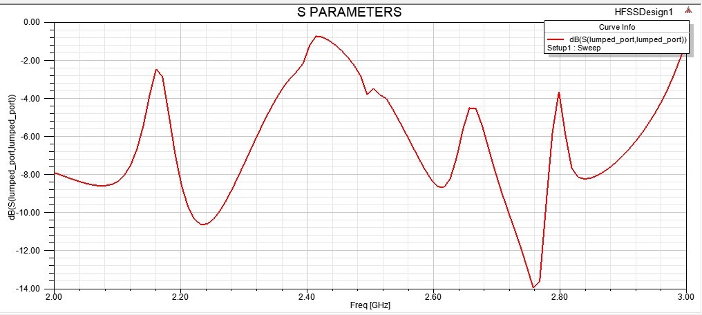
• The Y Parameters of the Dipole Antenna

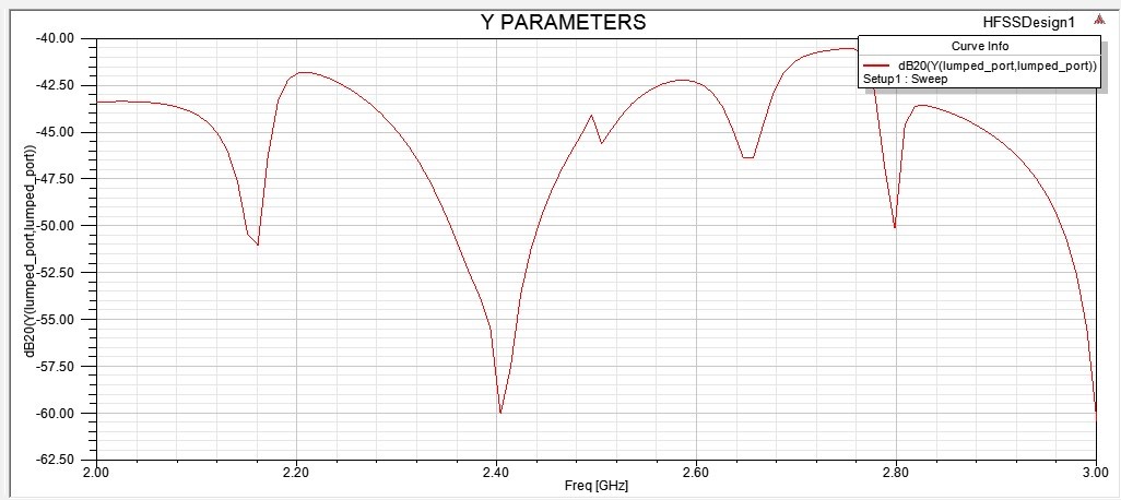
• The Z Parameters of the Dipole Antenna

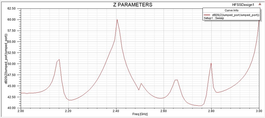
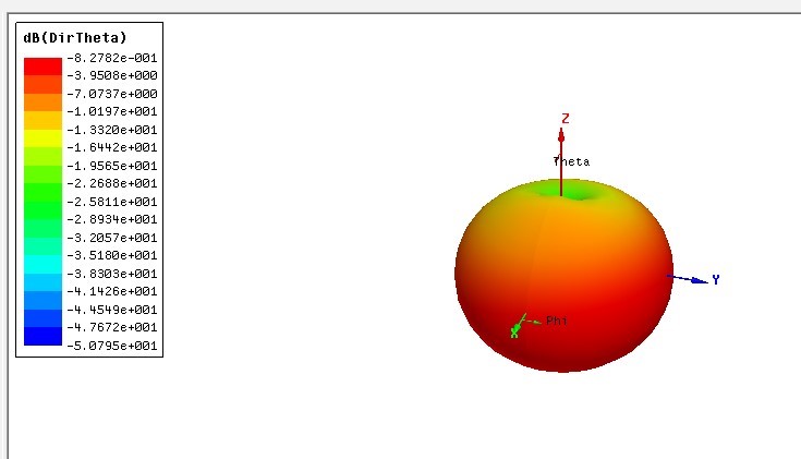
• The 3D Polar Plot (Db Dir Theta) of the Dipole Antenna Structure

• The 3D Polar Plot (Gain Theta) of the Dipole Antenna Structure

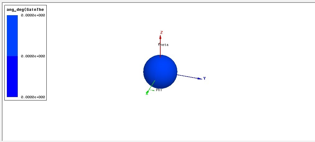
• The 3D Plot of the Radiation Pattern (with Total Gain)

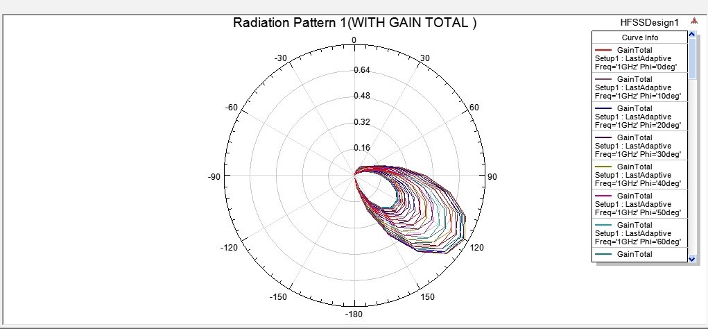
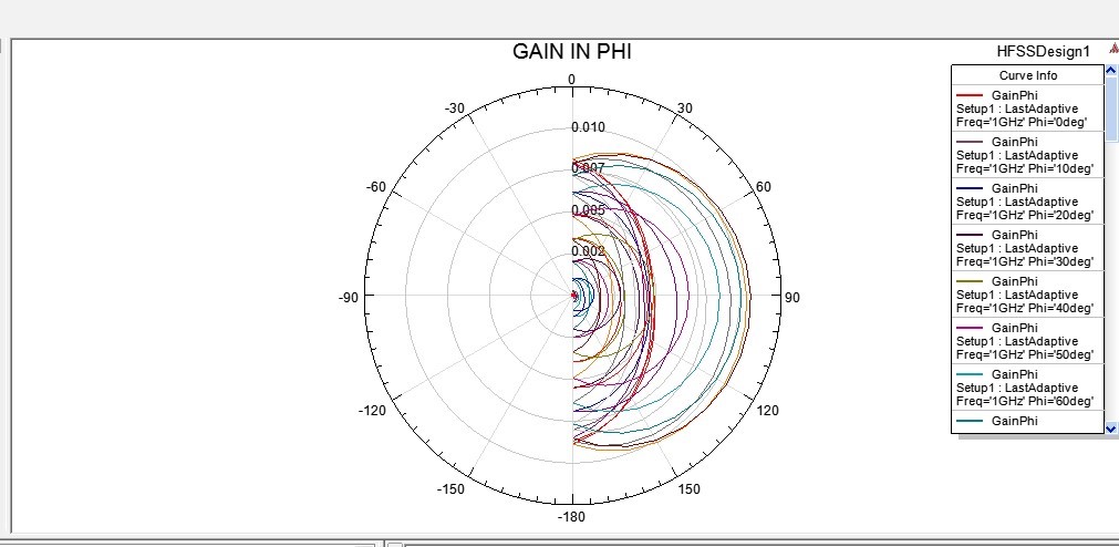
• The 3D Plot of the Gain in Phi of the Dipole Antenna

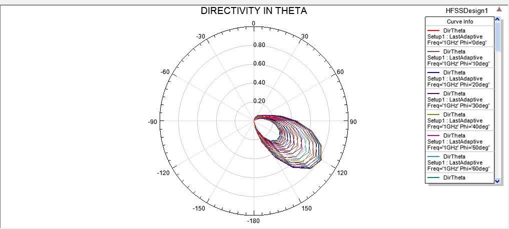
• The 3D Plot of the Directivity ( in Theta) of the Dipole Antenna

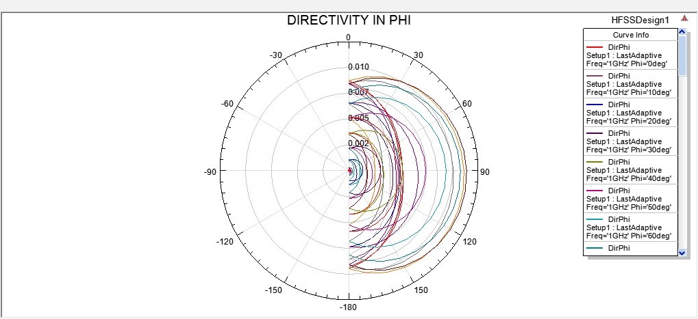
• The 3D Plot of the Directivity in Phi of the Dipole Antenna

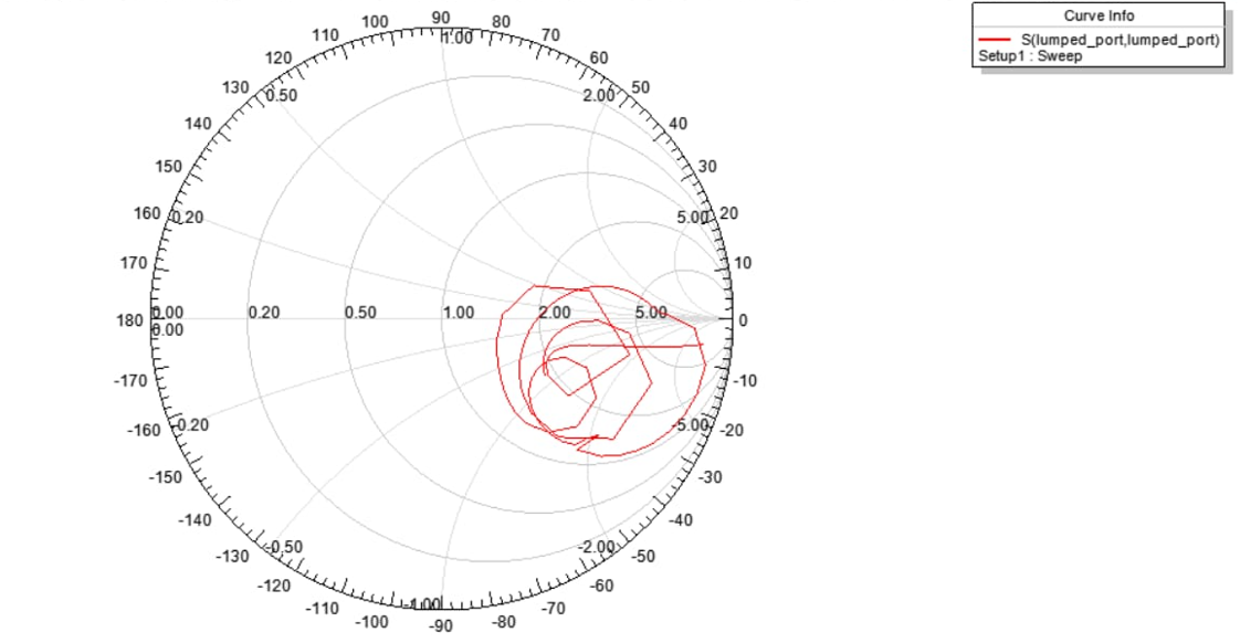
• Smith Contour Chart

It is a polar chart of S- parameters upon which a normalized impedance grid has been super imposed.

VERIFICATION OF PARAMETERS BY USING MATLAB:

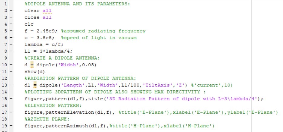
MATLAB code for Dipole Antenna 

%DIPOLE ANTENNA AND ITS PARAMETERS:

clear all

close all

clc

f = 2.45e9; %assumed radiating frequency

c = 3.8e8;  %speed of light in vacuum

lambda = c/f;

L1 = 3*lambda/4;

%CREATE A DIPOLE ANTENNA:

d = dipole(‘Width’,0.05)

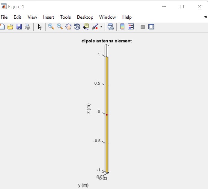
show(d)

%RADIATION PATTERN OF DIPOLE ANTENNA:

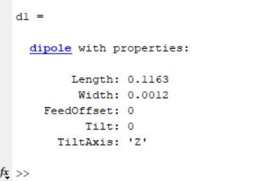
d1 = dipole(‘Length’,L1,’Width’,L1/100,’TiltAxis’,’Z’) %’current’,10)

%PLOTTING 3DPATTERN OF DIPOLE ALSO SHOWING MAX DIRECTIVITY :

figure,pattern(d1,f),title(‘3D Radiation Pattern of dipole with L=3\lambda/4’);

%ELEVATION PATTERN:

figure,patternElevation(d1,f), %title(‘E-Plane’),xlabel(‘E-Plane’),ylabel(‘E-Plane’)

%AZIMUTH PLANE:

figure,patternAzimuth(d1,f),%title(‘H-Plane’),xlabel(‘H-Plane’

• MATLAB SCREEN:

• COMMAND WINDOW:

It shows the Plot properties of the Dipole Antenna.

• OUTPUT SCREENS:

• Dipole Antenna Element:

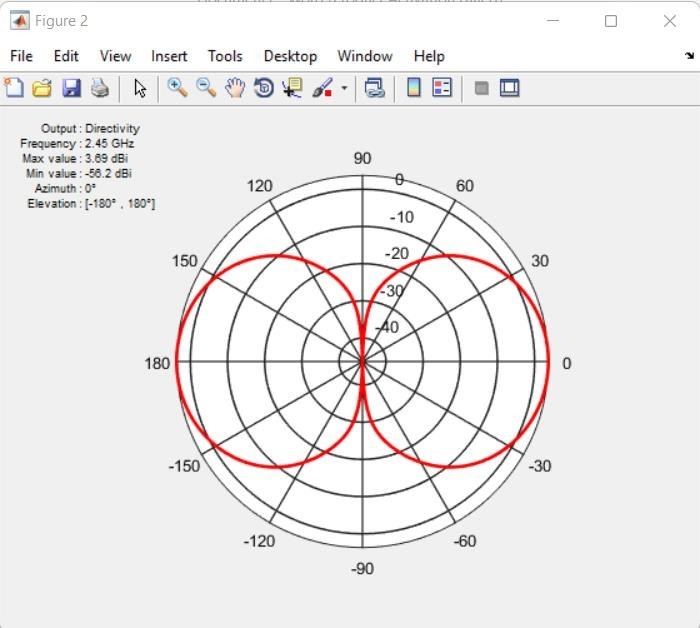
• Radiation Pattern of Dipole Antenna 

Azimuth Pattern of Dipole Antenna 

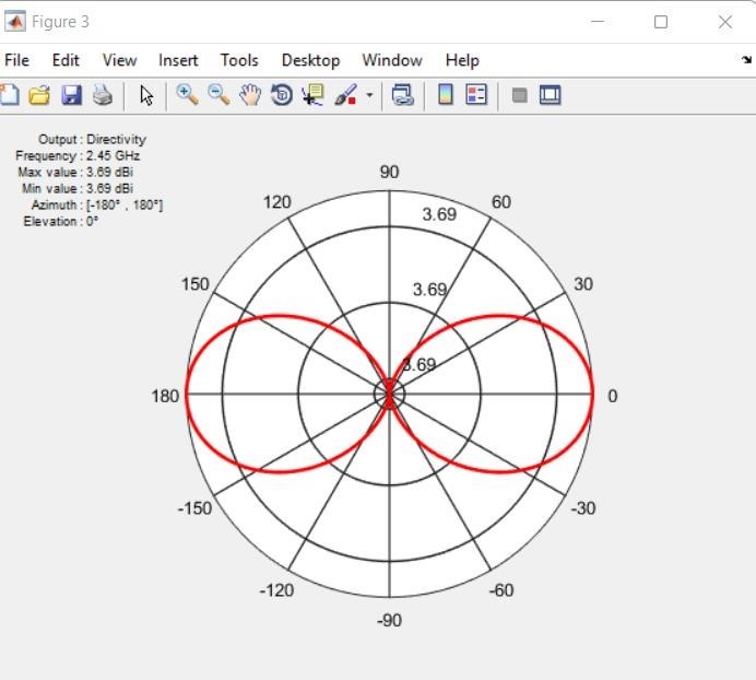
Elevation Pattern of Dipole Antenna 

• Impedance of the Dipole Antenna:

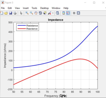
Note:

The impedance plot for the specified frequency of 2.4GHz will be attained from the MATLAB. As, it was more complex in HFSS. Moreover, we can verify the simulations too.

What are the Advantages of Dipole Antenna?

The below are some benefits of a dipole antenna:

• The fundamental benefit of this antenna is its compactness.
• When utilised at the resonance frequency, these are very effective.
• The efficiency of the dipole is unaffected by the separation formats
• When sending and accepting signals, they are omnidirectional.
• Telescoping dipoles provide you access to a greater frequency range than telescoping monopole antenna.
• The antenna is positioned in the hole’s center, giving this antenna a donut-shaped radiation pattern.
• Sloping, drooping, inverted V, and other configurations of these antennas are easy to build and operate.
• Almost every signal might be accepted regardless concern for direction.
• A loading coil may be utilized to decrease and resonate these antennas. We can achieve decent results when this coil is placed in the center.

What are the Applications of Dipole Antenna?

• Radio astronomy, satellite communications, and a variety of radio communication channels all use parabolic reflector-type dipole antennas.
• These antennas can function as the radiating element in various applications and are employed as a fundamental component in more complex antennas.
• Because the input impedance of a folded type dipole antenna is large, it may be matched simply by the transmission line impedance, allowing it to be utilised in various antennas for receiving worldwide TV signals across balanced lines.
• Radio and telecommunications uses this antenna.
• In two-way communication, the dipole antenna is utilised for receiving and sending.
• TV and radio receivers can use a half-wave type dipole antenna.
• Land mobile communications for public safety, coastal areas, industrial, and public communication applications primarily use VHF and UHF type dipole antennas.
• A dipole antenna is typically utilised as either a transmitting or receiving antenna because a receiving antenna can be used to convert electric signals into EM signals. A receiving antenna turns electromagnetic signals into electrical ones and transmits them in all direction.
• FM type dipole antennas are typically employed as FM broadcasting-receiving antennas, particularly for the FM broadcast band, which spans from 88 MHz to 108 MHz.

What is the Difference Between Monopole and Dipole Antenna?

Both dipole and monopole antenna belong to the linear antenna category. Following are the contrasts among the two:

• A monopole antenna requires a physical ground plane, whereas a dipole antenna just employs a radiator to create a synthetic ground plane in between the components of a symmetric radiator.
• In a monopole antenna, the outer conductor of the coaxial cable serves as the ground plane, but in a dipole antenna, the radiator components are simply linked to a conductor in a coaxial cable in 180-degree out-of-phase with one another.
• The monopole antenna exhibits the same performance & radiation patterns, but they are vertically symmetrical, in contrast to the dipole antenna, which exhibits the same performance & radiation patterns but not symmetrical radiation patterns.
• The ground plane orientation mostly affects the radiation pattern of monopole antennas whereas dipole antennas have a vertically symmetric radiation pattern, making it easy to point them in the optimal reception/transmission direction.
• There are many various forms of dipole antennas, including folded, short, common half-wavelength, etc., and many different types of monopole antennas, including automotive AM antennas and naval low frequency antennas.
• While monopole antennas are utilized in cordless phones, cellular, CB radios, walkie-talkies, etc., dipole antennas are used in a variety of applications as either an independent antenna or as a part of an antenna.

Conclusion

Simulation of the dipole antenna and analyzation of various parameters of its plot proves its importance in the domain of Electromagnetic field theory. We learned a lot about the working of the HFSS software as well as the construction of the antenna. The 3D polar plotting of the radiation patterns, efficiency plot, gain and directivity (theta and phi) provides us the accurate visualization of the working of dipole antenna and its parameters.

Dipole antenna is the most efficient radio frequency (RF) antenna, with the highest gain and efficiency level. That’s why it has vast range of applications specifically it proves to be effective in telecommunication domain.

Also Read here:

Implementation of Dipole Antenna using CST Microwave Studio