Interval arithmetic multiplier for digital signal processing
In this article I have discussed the design of an interval arithmetic multiplier for digital signal processing. Interval methods offer quite new research aspects regarding Digital Signal Processing. In scenarios like finite numeric representation, limited precision sensors or the quantization process, signal processing has been practicing interval mathematics as quite a reliable gizmo for expressing the uncertainties. Some types of control systems like estimating or soft computing systems, the uncertainties are caused due to the presence of variable instability, variance of signal, or the rate of safety of some actuators.
Since most DSPs are designed to work in real time environments, effective implementation of interval arithmetic for these processors asks for fast processing capabilities. Hence the aim is to develop an environment that facilitates interval arithmetic operations to be executed at the very same computational speed as is offered in many contemporary signal processors. So we are proposing the design and implementation of Interval Arithmetic multiplier that functions with IEEE 754 numbers. how to design an interval arithmetic multiplier for digital signal processing?
This design carries out the execution of an algorithm which performs better than conventional algorithm of Interval multiplier. The performance of proposed architecture is better than that of a conventional Canonic sign digit (CSD) floating-point multiplier, as it can perform interval multiplication and floating-point multiplication as well as Interval Comparisons.
What is interval arithmetic?
Applications associated to control, communications, multimedia, etc., have been employing digital signal processing because of high functionality and performance it attains for applications involving limited instruction set for implementing repetitive linear operations such as addition, multiplication, delay, etc., on a stream of sampled data. To fulfill the cost and performance needs of a particular application, digital signal processors have been combined with one or more FPGA devices or employed as attached coprocessor. One of the attractive aspects of digital signal processors is performing multiply-accumulate operations in a single instruction cycle. This operation is the basic step for performing vector product which is the key to computing digital filters, Fourier transforms and correlation. Underlying many of these is the need for accurate and reliable results, but errors can lead to inaccuracies. There are basically three different sources of error associated with numerical computations.
Define Data Problem
It occurs due to the fact that some given parameter values may not be known exactly (i.e. true for physically determined parameter values), or else they may not be exactly represented in a computer (i.e. the number π). Consider the expression f (x) = 1−x+ x2/2 with x = 0.531, i.e. with 10-3 precision. Computing this expression with classical arithmetic gives the result f (x) = 0.610. Now, if we perform he computations using IA, we get f (x) = 0.469 + 0.5312/2 ∈ 0.469 + [0.281,282]/2 and so f (x) ∈ 0.469 + [0.140, 0.141] = [0.609, 0.610]. Through this method it is made sure that the interval [0.609, 0.610] contains the exact answer. So we are very close to understand Interval arithmetic multiplier for digital signal processing.
- Truncation Error: occurs due to the necessity to terminate some infinite converging process after a finite number of steps. Or by the requirement that some well-defined expression is evaluated at some point whose location is known only approximately (i.e. the reminder term of Taylor series).
- Round-off Error: is caused by the necessity to restrict computational processes to operate on numbers which do not exceed some predetermined number of digits in length. It is the difference between the calculated approximation of a number and its exact mathematical value. It has traditionally been the most troublesome, primarily because of its non-analyticity.
Interval Arithmetic is a methodology which is used to examine and control numerical errors in computers. Ramon E. Moore published the first book on the subject entitled “Interval Analysis” in 1966. In the 1990’s, the interval arithmetic community observed substantial emergence and nowadays problems like global optimization, numerical analysis and many engineering and CAD issues, are being solved by utilizing interval algorithms.
Interval based algorithms continually keep on being answer to many signal processing and controls problems. For example, finding the optimal solution to a problem is often quite necessary in signal processing, i.e., cost function minimization.
The fact that makes the techniques of interval global optimization approaches quite fetching in DSP and control applications, is that they ensure convergence to global minimum point(s). Reliable results are interpreted as the solutions in which the outcome of the operation being executed is ensured to be exactly the accurate result. The interval established by interval analysis is guaranteed to contain the accurate answer expected from an operation executed on two input interval numbers. The principal advantage of traditional interval arithmetic is its ability to furnish the range of all the possible results of a given operation.
As many of the applications in DSP include tasks that are recursive and manipulate a sequence of data, hence there is always a chance of errors and uncertainties growing unboundedly over time. Utilization of interval arithmetic in such applications keeps the errors within limits. Better performing algorithms are established from the utilization of interval arithmetic due to its practice of:
- Eliminating instabilities occurring due to mathematical operations of numbers of very different order of magnitude, by monitoring certain parameters of the optimization algorithm
- Limiting the results to lie within certain bounds.
- Ensuring the convergence of the algorithm towards a stable filter by limiting the parameter space to certain bounds.
Slower computational speed is the main disadvantage in employing this algorithm in software. This happens because of the reason that interval arithmetic deals with two numbers instead of just one i.e. to operate on intervals.
Implementation of interval arithmetic in software experiences the disadvantage of additional overhead resulting from error and range checking, rounding modes, function calls and memory management. As a consequence, interval algorithms faces the weakness of experiencing relatively high execution time on contemporary computers, as compared to real arithmetic their counterparts.
To subdue the overhead experienced because of rounding, a hardware solution is mandatory that can perform the rounding calculations for each interval simultaneously. Interval Arithmetic Logic Units (I-ALU) are designed particularly to serve the purpose of operating on interval numbers. Any digital signal processor finds this type of an Interval ALU (I-ALU) attractive to be used as its core. The throughput of this ALU is desired to be comparable to that of non-interval units. DSPs are aimed to support the execution of algorithms that are characterized by repetitive multiply-and add operations, in contrast to the common general purpose microprocessors that are supposed to manage general computing operations. They utilize a modified Harvard architecture supporting separate data and program memory. how to design an interval arithmetic multiplier for digital signal processing?
Generally, capital letters are used for representing intervals and small letters are used for representing real numbers. The upper and lower interval end points of an interval X are represented as xu and xl, respectively. Any closed interval X= [ xl , xu] contains all the real numbers that lie in-between and including the two endpoints xl and xu (i.e., X={x: xl < x < xu}) as well. When arithmetic operation is performed on computer, it may not be possible to represent one or both end points of interval.Interval methods offer quite new research aspects
In this case, outward rounding is used for computing the interval endpoints. Outward rounding is performed by rounding the lower endpoint towards negative infinity (Ñ), and rounding the upper endpoint of the interval towards positive infinity (D), i.e. increasing the bound of the interval. While rounding towards negative infinity is called round down technique and rounding towards positive infinity is called round up technique. Outward rounding ensures that the resulting interval encloses the correct result. Addition, subtraction, multiplication, and division (basic arithmetic operations) are described for interval numbers as follows:
- Z=X+Y= [xl+yl,xu +yu]
- Z=X-Y= [xl-yu, xu – yl]
- Z= X*Y= [min (xl*yu, xl*xu , xu*yu, xu*yl), max (xl*xu, xu*yl, xu*yu, xl*yu)]
- Z= X/Y= [min (xl/yu, xl/xu, xu/yl, xu/yu), max (xl/xuxu/yl, xu/yu, xl/yu,)]
Previously implementation of interval arithmetic was performed in software. Slow speed was the main drawback of software implementation. They experienced large number of overhead due to the facts like function calls, changing of rounding modes, memory management, exception handling. For instance, multiplication operation requires large number of conditional branches to make the decision between the endpoints for multiplication to produce the proper required result. It is shown in the Table 1.
| Case | Condition | Z |
| 1 | xl>0, yl>0 | Zl=xlyl,Zu=xuyu |
| 2 | xl>0,yu<0 | Zl=xuyl, Zu=xlyu |
| 3 | xu<0,yl>0 | Zl=xlyu, Zu=xuyu |
| 4 | xu<0, yu<0 | Zl=xyyu, Zu=xlyl |
| 5 | Xl<0<xu, yl>0 | Zl=xlyl, Zu=xuyu |
| 6 | Xl<0<xu, yu<0 | Zl=xuyl, Zl=xlyl |
| 7 | Xl>0, yl<0<yu | Zl=xlyl, Zu=xuyu |
| 8 | Xl<0, yl<0<yu | Zl=xlyu, Zu=xlyl |
| 9 | Xl<0<xu,yl <0<yu | Zl=m n, Zu=m x |
Table1. Cases for interval multiplication
As we can see, for selecting the end points, depending on the values of the input intervals with respect to zero, nine distinct cases are to be considered for multiplication. In order to select between the multiplications cases, large number of conditional statements was needed. As individual operations were performed sequentially, extra work is done and it involves several time-consuming steps. In case of the misprediction of conditional branches, the performance penalty to be paid for was quite heavy in fully pipelined processors. Quite a large number of computational cycles are needed to change the rounding modes in software.
A numerous cycles delay and sever limitations in parallel execution are experienced due to the fact that changing of rounding mode on many processors requires the complete floating-point pipeline to be flushed. General implementation of interval multiplication in software is carried out through subroutines, and so due to several subroutine calls and returns, an extra overhead is faced during execution. Hence, contemporary computer architectures face the drawback of causing slower execution of interval algorithms as compared to that for their counterparts in real arithmetic . It was observed that software implementations turn out to perform almost four times slower than the executions performed by functionally equivalent hardware. how to design an interval arithmetic multiplier for digital signal processing?
In order to overcome these performance drops caused by software limitations, hardware support was employed. An ALU design based on interval was proposed to provide almost the same computational execution time for interval operations as that is provided in many DSPs. In this design there were two independent modules working in parallel to compute the lower and upper bound of the output interval. A particular functional unit of the ALU was designed to support the execution of the basic fixed-point interval arithmetic operations of addition, subtraction, multiplication along with the interval set operations of union and intersection. Another plus point is that through the multiply-accumulate instruction; the ALU was improved to perform dot products. Conventionally, division can only be implemented through shift operations on DSPs. In this design, division was done by shifting. The goal to achieve was to design ALU in order to have maximum throughput while diminishing area. The objective of this design was to solve DSP field problems with improved accuracy and faster rate.
what is Interval Arithmetic Multiplier?
The most general definition of interval(X= [xl,xu] and Y=[yl ,yu] ) multiplication is :
Z=X.Y= [min (xuyl,xlyl, xlyu, xuyu), max(xlyu ,xuyl, xuyu ,xlyl )]
If the floating point multiplier can provide at least two times of the accuracy in the inputs operands, in the resulted product, the interval multiplication can be calculated as:
Z=X.Y= [ min (xlyl, xlyu ,xuyl, xuyu), Δmax(xlyl, xlyu ,xuyl, xuyu)]
where and Δ represents rounding down and up towards negative and positive infinity respectively. According to this definition, calculating the endpoints of interval of Z involves four multiplications, four comparison operations, and two steps of fixed rounding. Normally interval arithmetic is still being practiced to perform on double precision input operands in order to produce a double precision output. In such case, X.Y can be calculated as:
Z=X.Y= [min ( xl.yl, xu.yl, xl.yu, xu.yu), max(Δ xl.yl, Δ xl.yu , Δ xu.yl, Δ xu.yu )]
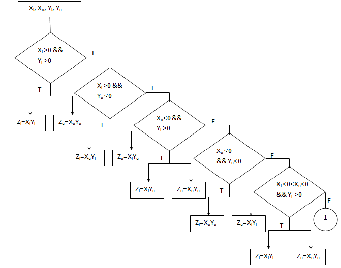
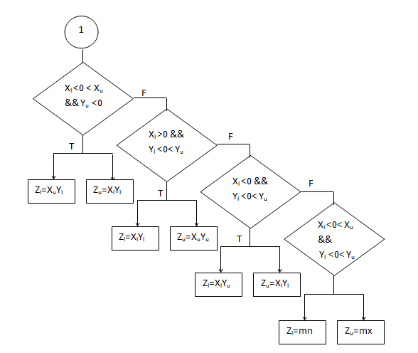
According to this definition, the interval endpoints of Z are calculated by doing eight multiplications, and six comparison operations. By employing the different technique, the number of multiplications can be reduced. This approach requires inspection of the signs of endpoints of the given intervals in order to make a decision of which endpoints should be multiplied to obtain the proper result. The endpoints signs of the intervals X and Y state the comparison of the numbers with zero i.e. whether X and Y are less, greater or do they contain zero within their intervals. This gives nine possible cases, as shown in the Figure 1.
how to design an interval arithmetic multiplier for digital signal processing?
The first eight cases require only two multiplications of floating-points to be performed. However, in the ninth case (when both intervals contain zero) only the sign bits inspection is not enough to determine the endpoints that are to be multiplied. One approach for dealing with this case is letting the interval multiplier handle it automatically on its own conditions. However, this method involves a substantial amount of extra hardware for storing the temporary values and calculating the minimum and maximum among them to decide the output. Control logic also gets complicated by this. Large numbers of conditional statements are employed to select among the nine cases, this causes the execution time of interval multiplication to increase. As this case arises seldom, the approach described in this paper includes four multiplications of floating points and four comparisons of the products obtained. The main drawback of such an algorithm is the difficulty in implementing it with pipelined structure due to the fact that the numbers of multiplication steps varies from case to case.
We propose new algorithm to evaluate the result for interval arithmetic multiplication shown in Table 2.
| P=xlyl | Min1=min(p,q) |
| q=xlyu | Max1=max(p,q) |
| R=xuyl | Min2=min(min1,r) |
| T=xuyu | Max2=max(max1,r) |
| Zl=min(min2,t) | Zu=max(max2,t) |
Table 2.Efficient Algorithm used for interval multiplication
*mn= min ( xlyu , xuyl)
*mx= max ( xlyl, xuyu)
It has much less calculations than the conventional interval multiplication shown in Figure 1. Two stages are involved in Interval Multiplication. In stage1 evaluation, product of two 64 bit double precision IEEE 754 floating point numbers is obtained. The following result for stage 1 is obtained, i.e. p=xl.yl, q=xl.yu, r=xu.yl, t=xu.yu, shown in figure 2. In stage 2 calculations, we find the minimum and maximum values of compared results of p, q, r & t, and then store the final result of multiplication in Zl and Zu registers.
Minimum1 and maximum1 values are obtained by comparing p and q during stage 2. Also by comparing minimum1 and r, minimum2 and maximum2 values are obtained. Finally we get Zl and Zu by comparing minimum2 and t. The final result is stored in Zl and Zu registers, shown in Figure 3. With this approach, we need only three floating-point comparisons and four floating-point multiplications to obtain result of interval multiplication. But conventional interval multiplication involves nine cases to verify which consume more time and hardware.
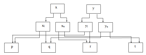
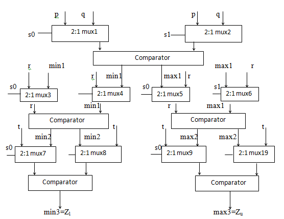
Figure 3 shows the stage 2 evaluation of interval multiplier. The calculated values of p,q and r,t are used as input to mux1 and mux2 respectively. P and q are selected and passed to 64 bit comparator when select line is (s0, s1) “0”. When select line is “1”, r and t are selected and passed to 64 bit comparator. The comparator produces the min1 and max1 values, min1 along with r is given to mux3 and mux4 respectively, max1 along with r is given to mux5 and mux6 respectively. how to design an interval arithmetic multiplier for digital signal processing?
The output of mux3 and mux4 (r, min1) are fed into 64 bit comparator and the output of mux5 and mux6 (r, max1) are fed into the 64 bit comparator. Select lines along with p, q are passed to mux5 and mux6 to evaluate minimum1 (min1) and maximum1 (max1) respectively. Next time select lines (s02, s12) becomes 01, minimum1 (min1) and r are selected from mux33 and mux4, passed to 64 bit comparator, resultant select lines(se13) along with minimum1 and r are fed to mux7 to get minimum2 (min2) value. Now select line (s02, s12) become 10 and minimum2 (min2) and t are passed to 64 bit comparator, depending on select line (sel323) and minimum2 (min2), t the result minimum3 (min3) is obtained through mux9 which is stored in Zl. now select line is (s02, s12) made 01, maximum1 (max1) and r are selected through multiplexers 3 and 4, and passed to 64 bit comparator. 3 bit select line (sel321) along with max1 and r are given to multiplexer (mux8) to obtain the result maximum2 (max2). Next the select line(s02, s12) becomes 10, maximum2 (max2) and t are selected through mux3 and mux4, passed to 64 bit comparator, compared, the resultant select line(sel322m) along with max2 and t are given to mux10 to get maximum3 (max3), the result maximum3 is stored at Zu. The result Z of interval multiplication is denoted as (Zl, Zu). By applying this algorithm, number of comparisons has been reduced to almost half of the required.
Performance Analysis
Efficiency is the basic purpose of any design or algorithm. One way to measure the efficiency is through the analysis of execution speed of the algorithm.
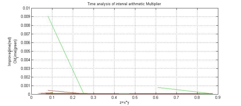
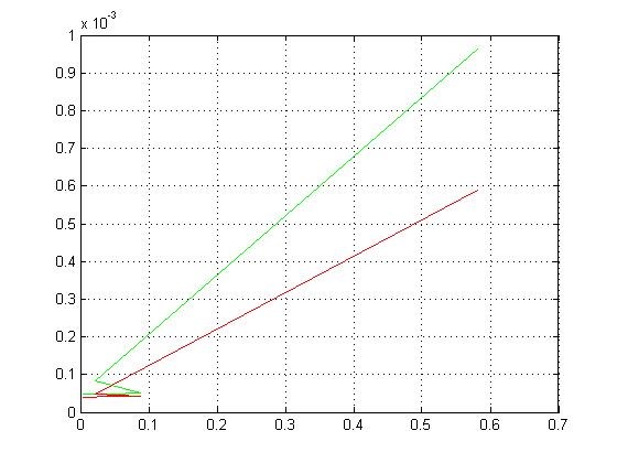
The algorithm we have described in the last section has been executed and analyzed on MATLAB for the multiplication of random numbers. We have compared the previous algorithm with our proposed algorithm on the basis of time taken for the execution of multiplication of some random numbers chosen by MATLAB. We observed that the time taken by the previous approach is comparatively higher than that of the newer approach, as demonstrated by the Figures 4a and 4b.We made a function in MATLAB that executes both the old and new algorithms of interval multiplication for the same set of numbers, generated randomly. Then calculates the time taken by both algorithms and plots them against each product on same graphs, old algorithm time shown in green color and new in red color in figures 4a and 4b. These are two graphs for two different set of numbers but both show that the new approach takes comparatively less time to calculate the output interval.
Conclusion & Future Directions
An effective way to design and implement interval arithmetic units is demonstrated in this paper, by proposing a new algorithm for interval multiplier that is aimed to be employed in the fields of DSP and control. The algorithm discussed here finds its application in multiplication of both intervals as well as floating-points.
Because of the execution of interval comparisons along with interval multiplication, interval multiplications are executed with better accuracy and performance as compared to formal floating point multiplication. To compute given any two Interval numbers, the proposed IA multiplier uses four multiplications and three comparisons, whereas for convention interval multiplication algorithm, with respect to cases the number of steps for the multiplication is not fixed, because of which pipeline implementation becomes difficult.
However, the hardware implementation of the proposed multiplier algorithm is a future prospect of our work, pipelining can be an efficient way to increase performance. Moreover the comparator can also be used for other important interval operations, such as interval hull and intersection. Efficient utilization of active area along with improved functionality and performance can be achieved this way.
Also read here
How to find the square root of a number using Newton Raphson method?