What is the interpolation
How many types of interpolation are there? Interpolation is the technique of determining the value or the expression of function from the given set of data points. If we are given some data and we want to determine the behavior or function according to which these data points are generated we can do this using interpolation techniques. When we want to determine the value of function within the range of given data points, it is called interpolation. When we want to determine the value of function outside the given range of data we call it as extrapolation.
How many types of interpolation techniques are here?
There are many techniques available for interpolation. The behavior of data points help to decide which technique to select. These techniques are listed below
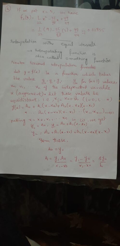
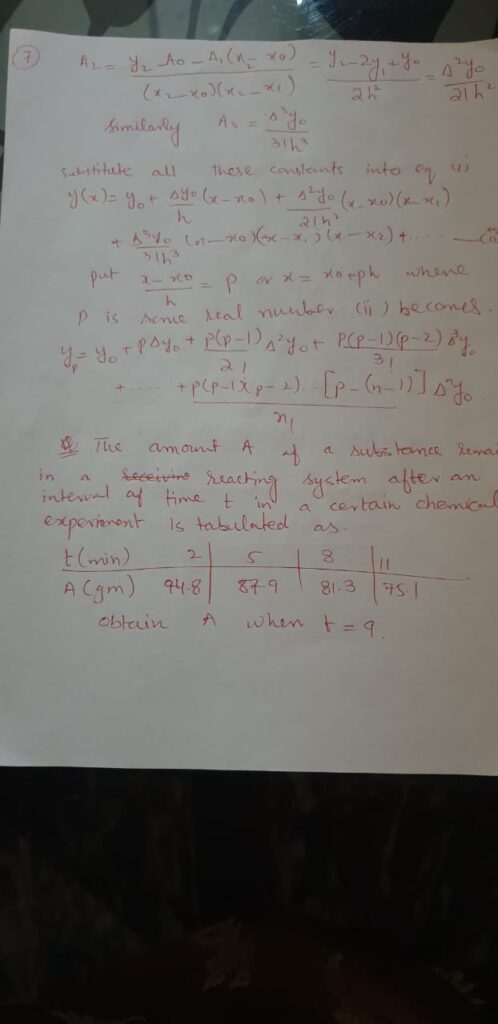
- Newton’s forward difference interpolation
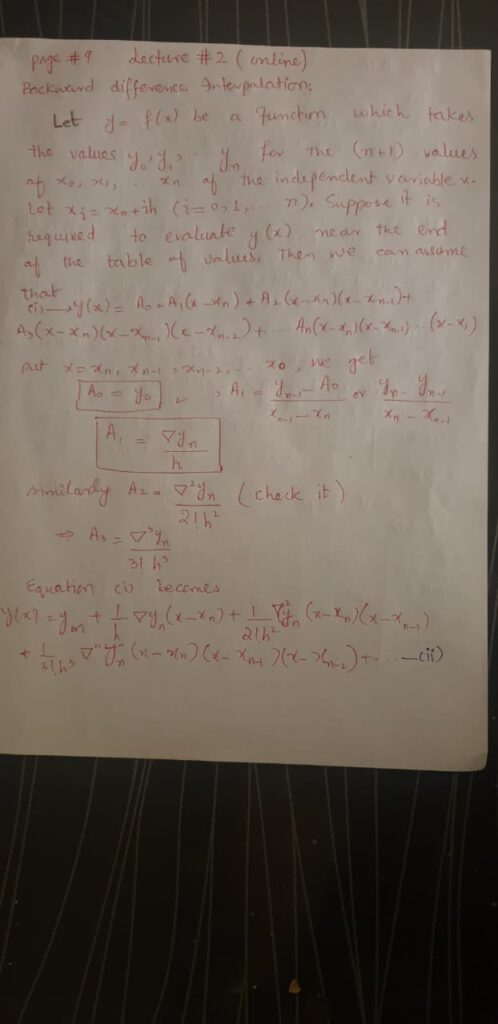
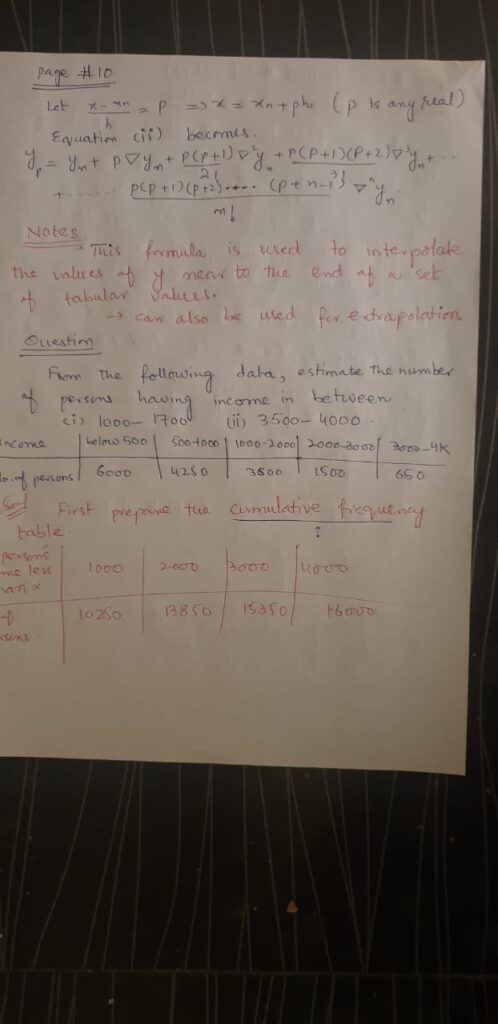
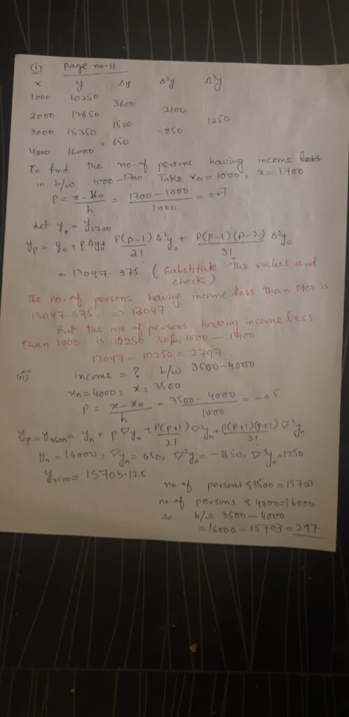
- Newton’s backward difference interpolation
- Newton’s divided difference interpolation
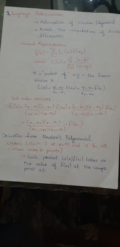
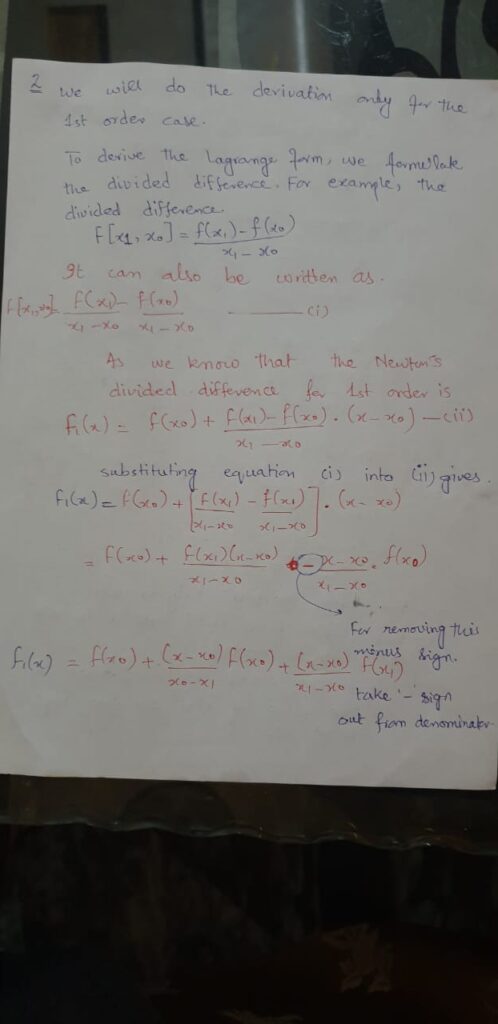
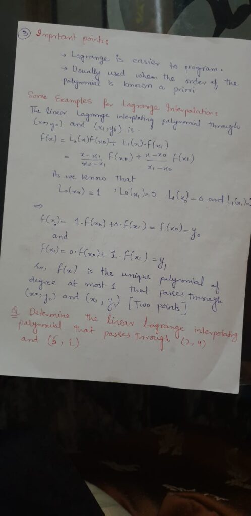
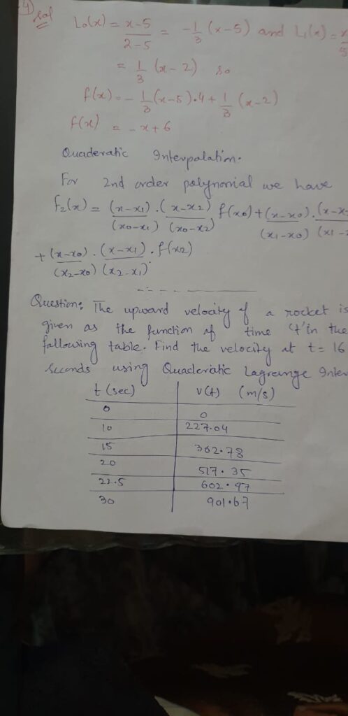
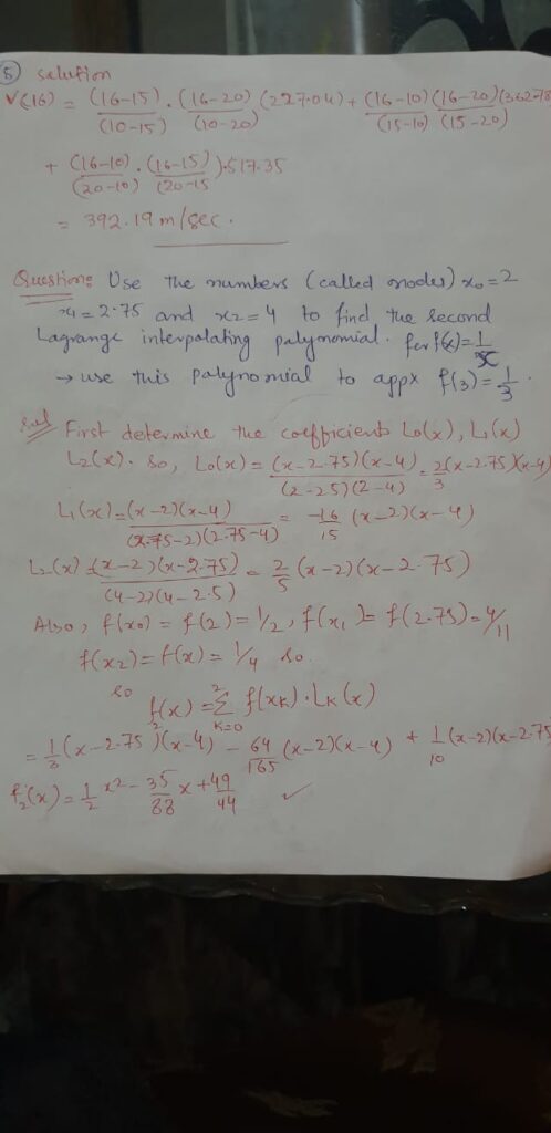
- Lagrange Interpolation Technique
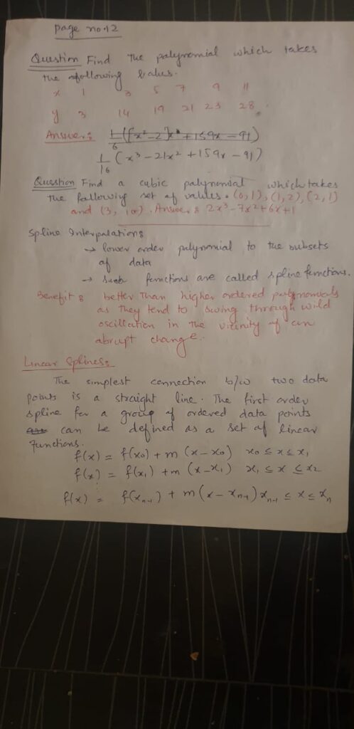
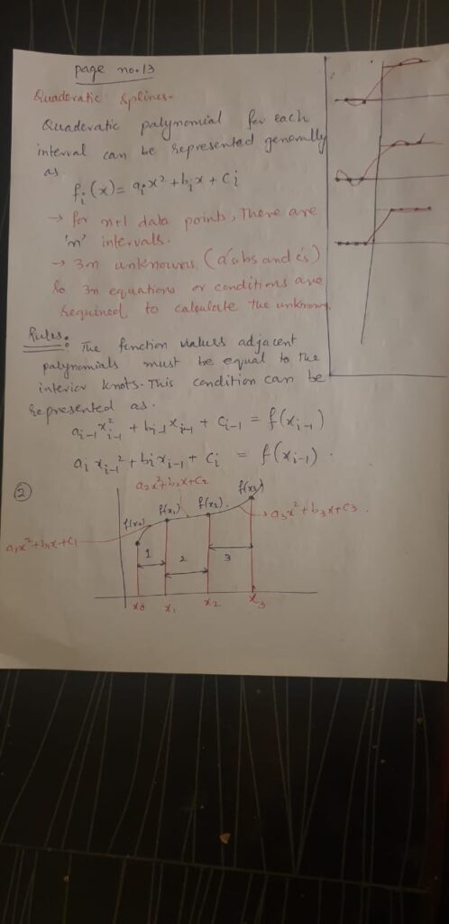
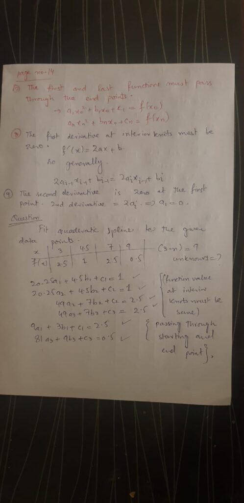
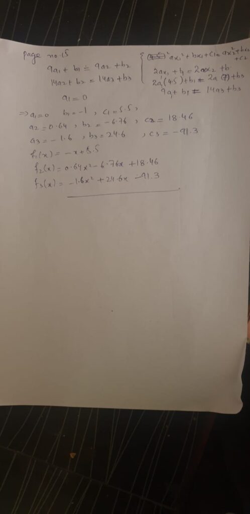
- Spline Interpolation
The choice of interpolation technique depends on the behavior of data points usually. If the data points are equally distant, then we can use any of these interpolation techniques. But if the data points are not equally distant then we can use Lagrange, spline or Newton’s divided difference interpolation technique. All these interpolation techniques are polynomial interpolation techniques. It means they all produce the output function in the form of a polynomial.
When should we use forward difference interpolation and backward difference interpolation?
If the data points are equally distant then we can use either the forward difference or backward difference interpolation technique. Now the question is which one to follow? If the point at which we want to determine the value of the function lies near the beginning of data points then forward difference interpolation technique should be used. If the point lies near the end of given data points then backward difference interpolation technique should be used. The reason is that as the data points increase, the oscillations in the polynomial increase which may result in some more erratic value. For n+1 data points we get the polynomial of ‘n’ degree. Lets consider the following case for understanding this concept.
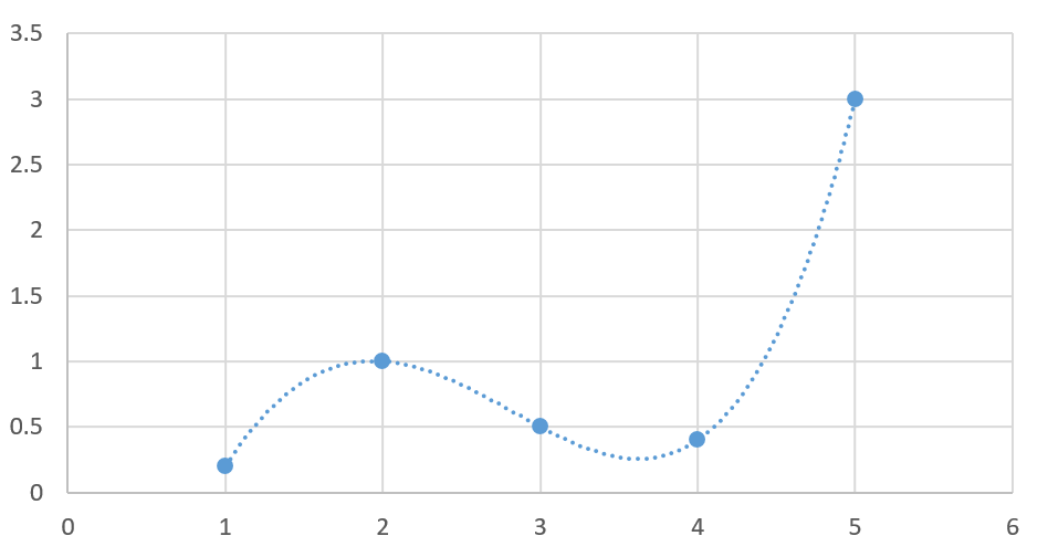
In the above figure, if we want to determine the value of the function at x=0.5, then we will prefer forward difference interpolation as it will cause less oscillations as can be seen. But if the backward difference interpolation technique is used then with the increase in order, the oscillatory result will be obtained.
What is the meaning of equidistance data points?
By the equidistance we mean difference between two consecutive data points (value of x )should be same or equal. So the given data points are equidistance.
| Data (x) | 0 | 1 | 2 | 3 | 4 | 5 | 6 |
| y=f(x) | 0 | 0.2 | 0.5 | 2 | 2.5 | 4 | 8 |
It can be seen the difference between any two values of x is same. Now consider the following data points where we can notice the data points are not equidistance.
| Data (x) | 0 | 1.5 | 2 | 3.5 | 6 | 9 | 20 |
| Y=f(x) | 0 | 0.2 | 6 | 2.5 | 7 | 4 | 8 |
Lets us discuss each type of interpolation with an example.
Newton’s divided difference Interpolation
This technique is used when the data points are random. As it is based on the concept of polynomial interpolation so it can be linear, quadratic, cubic or of any high order.
Linear Interpolation
Linear interpolation technique is based on the fact of joining two pints with a straight line as shown in the figure below
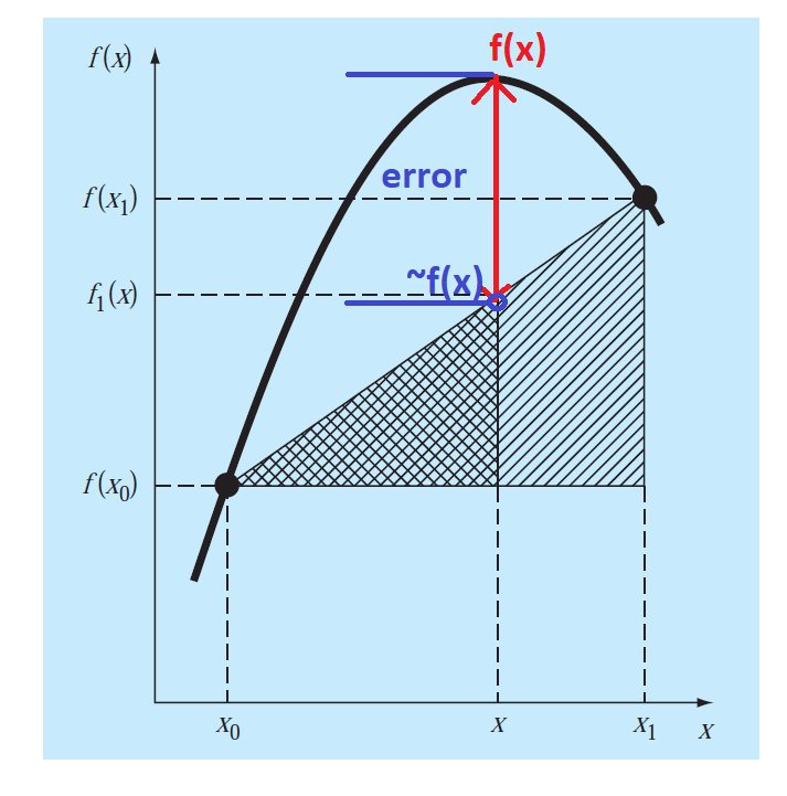
Lets say x is a point at which we want to determine the value of the function. The actual function is shown in the curved form. The value of f(x) at x is marked in red. While the interpolating function is approximating it with a straight line and its value is marked in blue ~f(x). The difference between actual value and approximated value of f(x) gives error.
Formula Derivation


The term f(x1)-f(x0)/x1-x0 is called finite-divided-difference.
Example of Linear interpolation
Estimate the value of ln(2) when you are given the value of ln(1)=0 and ln(4)=1.386294.
Solution:
| X | 1 | 4 |
| Y=ln(x) | 0 | 1.386294 |

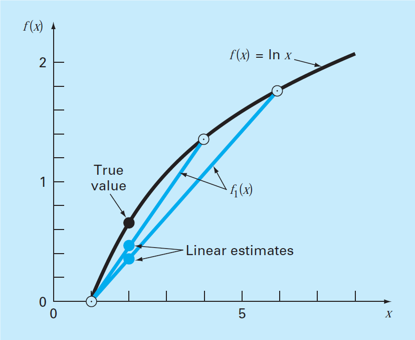
The approximated value of f(2)= 0.4620981. As we narrow down the interval, the accuracy increases. The following graph shows how the error reduces when interval is decreased.
Quadratic Interpolation
When we have three data points, then the quadratic interpolation can be used. In the previous example, it can be seen that we were trying to approximate the curve with a straight line. That’s why the error was large. In order to reduce the error it is preferable to approximate a curved behavior with some quadratic function or some parabola.
The general expression for quadratic interpolation is given below.
![]()
The subscript 2 in f(x) shows the order of the interpolation technique. Here b0,b1 and b2 are the coefficients to be determined. This is the general form of the quadratic equation and it can be seen later on how it will represent a quadratic equation. Now, the question is how to determine the value of these coefficients?.
If we substitute x0,x1,and x2=0 one by one we can determine the values of these coefficients. So when we put x0=0 the we get
f(x0)=b0
Similarly, we get the other coefficients


Once we determine the values of these coefficients, we can determine the value of function for any value of x.
Example of quadratic interpolation
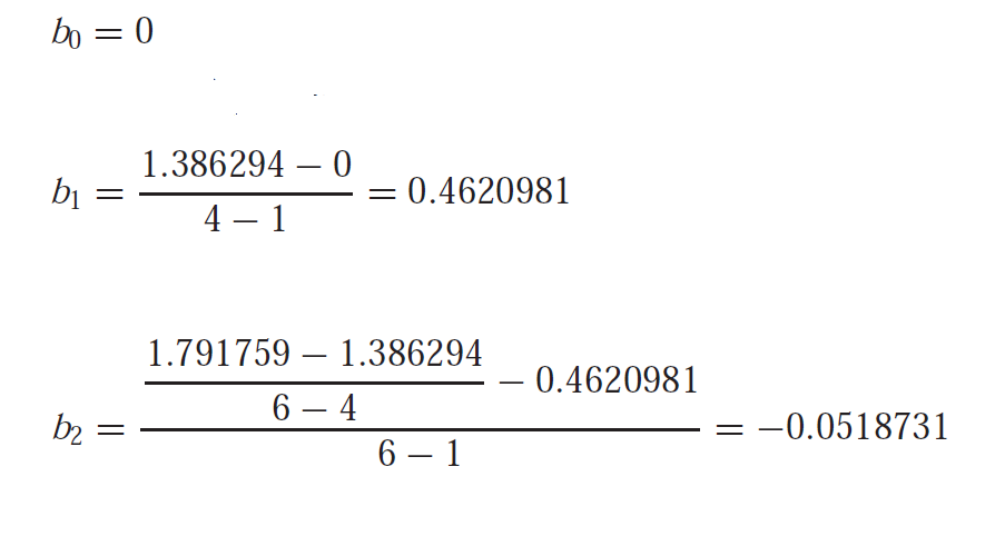
Lets consider again the case of determining the value of ln(2) for the given values of x and f(x) as shown below
| X | 1 | 4 | 6 |
| Y=ln(x) | 0 | 1.386294 | 1.791759 |
Solution
![]()
![]()
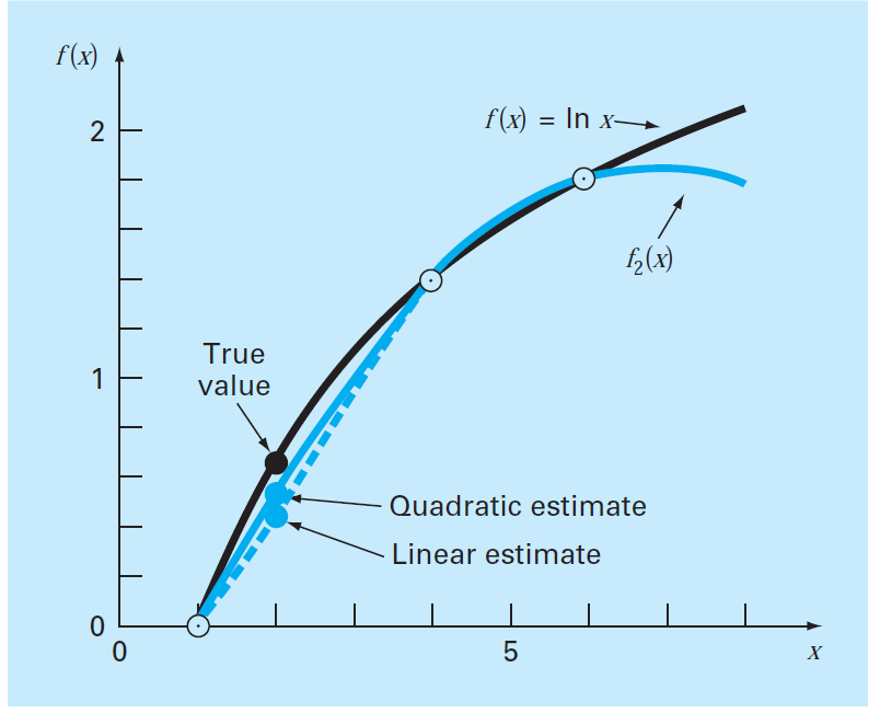
The above picture shows the graphical depiction how the quadratic interpolation gives better result as compared to liner interpolation. Hence the error is reduced.
General form of Newton’s interpolating polynomial.
For n+1 data points we can have polynomial of order n. The general form of it is given below:
![]()
Where , the coefficients are determined as the divided difference
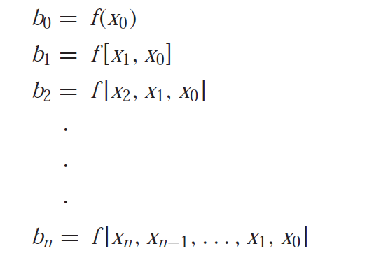
Generally the finite divided difference of any two numbers is represented as

For second finite divided difference we have

Similarly for nth finite divided difference
![]() The following picture shows the graphical representation of the recursive nature of divided difference formula.
The following picture shows the graphical representation of the recursive nature of divided difference formula.

These difference formulas can be substituted for calculating the value of function at any point x.

The above formula is known as Newton’s divided difference polynomial interpolation formula.
Also read here
https://eevibes.com/describe-and-develop-the-formula-for-newtons-forward-difference-interpolation/
watch here
One thought on “How many types of interpolation are there?”