The term critical value refers to a cut-off value utilized to indicate the beginning of an area in which the test statistic, as derived from hypothesis testing, is unlikely to fall. To decide whether or not to reject the null hypothesis, the critical value is compared with the test statistic that was produced.
In this comprehensive guide, we will explore the notion of critical value. We will explain hypothesis testing in different distributions with one-tailed and two-tailed. We will address these terms with the help of some examples.
Critical Value:
A critical value denotes a range of values that necessitate rejecting the null hypothesis, as indicated by a point on the test statistic’s distribution beneath the hypothesis itself. The critical or rejection region is what is known as this set.
If the calculated test statistic is more than what would be predicted if the null hypothesis were true, then using the critical value approach, one can determine if it is likely or unlikely to be. The test statistic that was observed is compared to a critical value, which is a cutoff number.
The alternative hypothesis is accepted and the null hypothesis (H0) is rejected if the test statistic is greater than the critical value. The null hypothesis (H0) is accepted if the test statistic is less than the critical value.
Kinds of Critical Value
Below are a few kinds of critical value.
Critical Value in F-Distribution:
In regression and variance analysis (variance analysis is represented as ANOVA), the F-critical value is essential. In a hypothesis test that involves variances, this sort of critical value elaborates on whether to reject or fail the null hypothesis (Ho). Typically, the notation Fα, df1, df2 is used to express it.
In this case, α stands for the significance level, and df1, df2, and the denominator represent the degrees of freedom, respectively.
The f-critical value is determined by identifying the alpha value (α) and subtracting it from the first sample size (it will be the degree of freedom represented as df1) as well as from the 2nd sample size (it will be the degree of freedom represented as df2).
Now determine the f-critical value by observing the intersection of the df1 and the df2 value in the f-distribution table.
Test statistic having a large sample:
f = (σ12 / σ22) where σ12 represents the variance for the 1st sample size and σ12 represents the variance for 2nd sample size.
Test statistic having a small sample:
f = (s12 / s22) ) here s12 represents the variance for the 1st sample size and s22 represents the variance for 2nd sample size.
Critical Value in Chi-Square Distribution:
Chi-squares are derived from two different kinds of chi-square tests: independence and quality of fit. A small sample of sample data can be used to assess whether it is representative of the entire population using the goodness of fit chi-square test.
To determine the relationship between two variables, you will compare them using the independence chi-square test. The sample data is compared to the population data using the chi-square test. Comparing two variables to determine their relationship is another usage for it.
A chi square critical value can be determined by identifying the alpha level (α) and subtracting it from the sample size (it will be the degree of freedom represented as df). Now determine the chi-square critical value by observing the intersection of the df and the α value in the chi-square table.
Calculations of Critical Value
Example 1
Consider an example where we want to find the critical value for an F-distribution with degrees of freedom (df_1 = 3) and ( df_2 = 5) at a significance level of (alpha = 0.10 ).
SOLUTION:
Step 1: Identify Degrees of Freedom:
(df_1 = 3)
(df_2 = 5)
Step 2: Determine Significance Level:
(alpha = 0.10)
Step 3: Use an F-distribution Table:
Look up the critical value in an F-distribution table using the degrees of freedom (df_1) and ( df_2) at the given significance level (alpha).
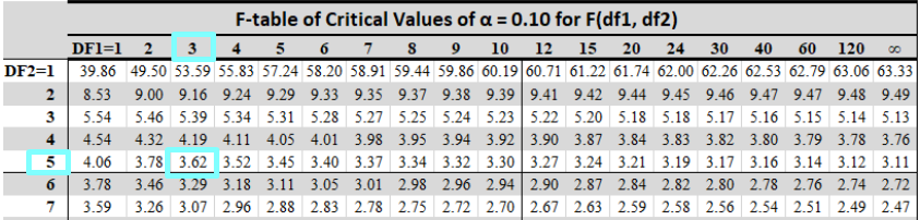
So,
F{critical} = 3.62 Ans.
Example 2:
Consider the F-distribution in the context of comparing the variances of two samples. Suppose we have two independent samples and aspire to test if their variances are significantly different for the following information:
Sample 1:
n1 = 16, s12 = 4.5
Sample 2:
n2 = 21 and s22 = 3.0
SOLUTION:
Step 1: Given information is:
Sample 1:
n1 = 16, s12 = 4.5
Sample 2:
n2 = 21 and s22 = 3.0
Step 2: Using Test Statistic:
Calculate the test statistic (F):
F = (s1^2 / s2^2)
F = (4.5/3.0)
F = 1.5
Step 3: Degrees of freedom:
Degrees of freedom for sample 1:
Df1 = n1 – 1 = 15 – 1 = 15
Degrees of freedom for sample 2:
Df2 = n2 – 1 = 20 – 1 = 20
Step 4: To compare the calculated F-statistic to critical values, we need to determine the critical region based on the chosen significance level (α). Suppose we choose α = 0.05 for a two-tailed test.
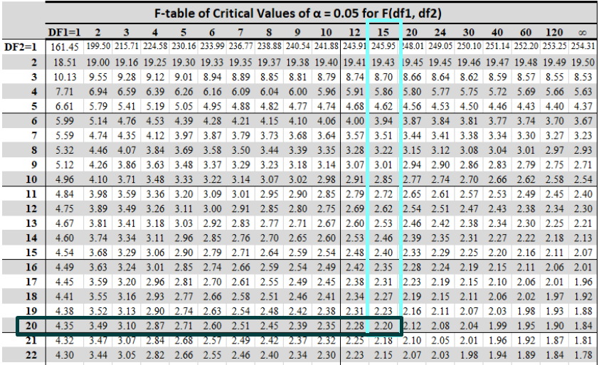
Using an F-distribution table, we find the critical values for df1 = 15 and df2 = 20 to be approximately 2.20
Decision:
We know that if F falls in the critical region (F < Fcritical, left or F > Fcritical, right), we are to reject the null hypothesis and if F does not fall in the critical region, fail to reject the null hypothesis. In our case, F = 1.5 does not fall in the critical region, so we fail to reject the null hypothesis.
This means we do not have enough evidence to conclude that the variances of the two samples are significantly different at the 0.05 significance level.
Wrap Up
In this comprehensive guide, we have discussed the important notion of critical value precisely. We have explored this notion in the f-distribution and chi-square distribution. We also addressed some examples to understand concisely.