This series will acquaint you with diagramming in python with Matplotlib, which is seemingly the most famous charting and information representation library for Python.
The least demanding method for introducing matplotlib is to utilize pip. Type following order in terminal:When envisioning information, frequently there is a need to plot numerous charts in a solitary figure. For example, numerous charts are valuable to picture a similar variable yet from various points (for example next to each other histogram and boxplot for a mathematical variable). In this post, I share 4 basic yet viable ways to plot different charts.
Pythonistas normally utilize the Matplotlib plotting library to show numeric information in plots, diagrams, and graphs in Python. A wide scope of use is given by matplotlib’s two APIs (Application Programming Interfaces):
Pyplot API interface, which offers an order of code protests that make matplotlib work like MATLAB.
OO (Object-Oriented) API interface, which offers an assortment of articles that can be collected with more prominent adaptability than pyplot. The OO API gives direct admittance to matplotlib’s backend layer.
The pyplot interface is simpler to execute than the OO form and is all the more usually utilized. For data about pyplot capacities and phrasing, allude to: What is Pyplot in Matplotlib
# importing the required moduleimport matplotlib.pyplot as plt# x axis valuesx = [1,2,3]# corresponding y axis valuesy = [2,4,1]# plotting the pointsplt.plot(x, y)# naming the x axisplt.xlabel('x - axis')# naming the y axisplt.ylabel('y - axis')# giving a title to my graphplt.title('My first graph!')# function to show the plotplt.show() |
Output:
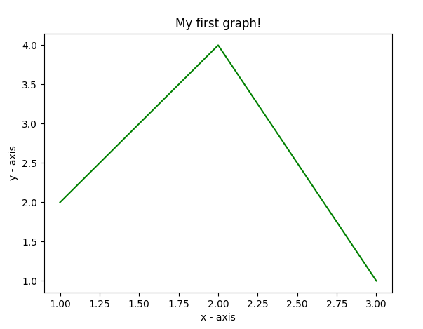
The code seems self-explanatory. Following steps were followed:
- Define the x-axis and corresponding y-axis values as lists.
- Plot them on canvas using .plot() function.
- Give a name to x-axis and y-axis using .xlabel() and .ylabel() functions.
- Give a title to your plot using .title() function.
- Finally, to view your plot, we use .show() function.
Plotting two or more lines on same plot
- Python
import matplotlib.pyplot as plt# line 1 pointsx1 = [1,2,3]y1 = [2,4,1]# plotting the line 1 pointsplt.plot(x1, y1, label = "line 1")# line 2 pointsx2 = [1,2,3]y2 = [4,1,3]# plotting the line 2 pointsplt.plot(x2, y2, label = "line 2")# naming the x axisplt.xlabel('x - axis')# naming the y axisplt.ylabel('y - axis')# giving a title to my graphplt.title('Two lines on same graph!')# show a legend on the plotplt.legend()# function to show the plotplt.show() |
Output:
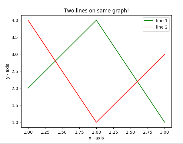
- Here, we plot two lines on the same graph. We differentiate between them by giving them a name(label) which is passed as an argument of the .plot() function.
- The small rectangular box giving information about the type of line and its color is called a legend. We can add a legend to our plot using .legend() function
Customization of Plots
Here, we discuss some elementary customizations applicable to almost any plot.
- Python
import matplotlib.pyplot as plt# x axis valuesx = [1,2,3,4,5,6]# corresponding y axis valuesy = [2,4,1,5,2,6]# plotting the pointsplt.plot(x, y, color='green', linestyle='dashed', linewidth = 3, marker='o', markerfacecolor='blue', markersize=12)# setting x and y axis rangeplt.ylim(1,8)plt.xlim(1,8)# naming the x axisplt.xlabel('x - axis')# naming the y axisplt.ylabel('y - axis')# giving a title to my graphplt.title('Some cool customizations!')# function to show the plotplt.show() |
Output:
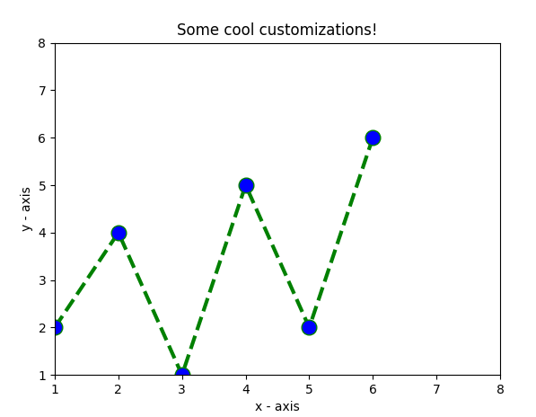
As you can see, we have done several customizations like
- setting the line-width, line-style, line-color.
- setting the marker, marker’s face color, marker’s size.
- overriding the x and y-axis range. If overriding is not done, pyplot module uses the auto-scale feature to set the axis range and scale
Bar Chart
- Python
import matplotlib.pyplot as plt# x-coordinates of left sides of barsleft = [1, 2, 3, 4, 5]# heights of barsheight = [10, 24, 36, 40, 5]# labels for barstick_label = ['one', 'two', 'three', 'four', 'five']# plotting a bar chartplt.bar(left, height, tick_label = tick_label, width = 0.8, color = ['red', 'green'])# naming the x-axisplt.xlabel('x - axis')# naming the y-axisplt.ylabel('y - axis')# plot titleplt.title('My bar chart!')# function to show the plotplt.show() |
Output :
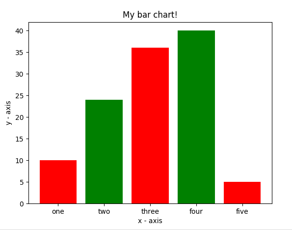
- Here, we use plt.bar() function to plot a bar chart.
- x-coordinates of the left side of bars are passed along with the heights of bars.
- you can also give some names to x-axis coordinates by defining tick_labels
Histogram
- Python
import matplotlib.pyplot as plt# frequenciesages = [2,5,70,40,30,45,50,45,43,40,44, 60,7,13,57,18,90,77,32,21,20,40]# setting the ranges and no. of intervalsrange = (0, 100)bins = 10# plotting a histogramplt.hist(ages, bins, range, color = 'green', histtype = 'bar', rwidth = 0.8)# x-axis labelplt.xlabel('age')# frequency labelplt.ylabel('No. of people')# plot titleplt.title('My histogram')# function to show the plotplt.show() |
Output:
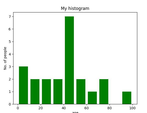
- Here, we use plt.hist() function to plot a histogram.
- frequencies are passed as the ages list.
- The range could be set by defining a tuple containing min and max values.
- The next step is to “bin” the range of values—that is, divide the entire range of values into a series of intervals—and then count how many values fall into each interval. Here we have defined bins = 10. So, there are a total of 100/10 = 10 intervals.
Scatter plot
- Python
import matplotlib.pyplot as plt# x-axis valuesx = [1,2,3,4,5,6,7,8,9,10]# y-axis valuesy = [2,4,5,7,6,8,9,11,12,12]# plotting points as a scatter plotplt.scatter(x, y, label= "stars", color= "green", marker= "*", s=30)# x-axis labelplt.xlabel('x - axis')# frequency labelplt.ylabel('y - axis')# plot titleplt.title('My scatter plot!')# showing legendplt.legend()# function to show the plotplt.show() |
Output:
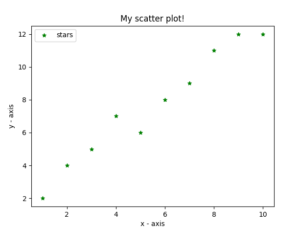
- Here, we use plt.scatter() function to plot a scatter plot.
- As a line, we define x and corresponding y-axis values here as well.
- marker argument is used to set the character to use as a marker. Its size can be defined using the s parameter.
Pie-chart
- Python
import matplotlib.pyplot as plt# defining labelsactivities = ['eat', 'sleep', 'work', 'play']# portion covered by each labelslices = [3, 7, 8, 6]# color for each labelcolors = ['r', 'y', 'g', 'b']# plotting the pie chartplt.pie(slices, labels = activities, colors=colors, startangle=90, shadow = True, explode = (0, 0, 0.1, 0), radius = 1.2, autopct = '%1.1f%%')# plotting legendplt.legend()# showing the plotplt.show() |
The output of above program looks like this:
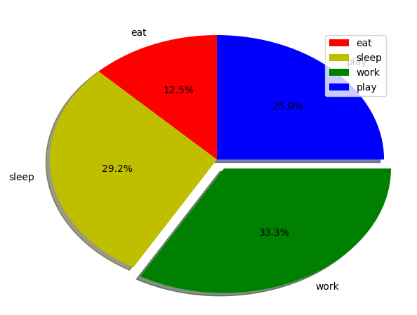
- Here, we plot a pie chart by using plt.pie() method.
- First of all, we define the labels using a list called activities.
- Then, a portion of each label can be defined using another list called slices.
- Color for each label is defined using a list called colors.
- shadow = True will show a shadow beneath each label in pie chart.
- startangle rotates the start of the pie chart by given degrees counterclockwise from the x-axis.
- explode is used to set the fraction of radius with which we offset each wedge.
- autopct is used to format the value of each label. Here, we have set it to show the percentage value only upto 1 decimal place.
Plotting curves of given equation
- Python
# importing the required modulesimport matplotlib.pyplot as pltimport numpy as np# setting the x - coordinatesx = np.arange(0, 2*(np.pi), 0.1)# setting the corresponding y - coordinatesy = np.sin(x)# plotting the pointsplt.plot(x, y)# function to show the plotplt.show() |
The output of above program looks like this:
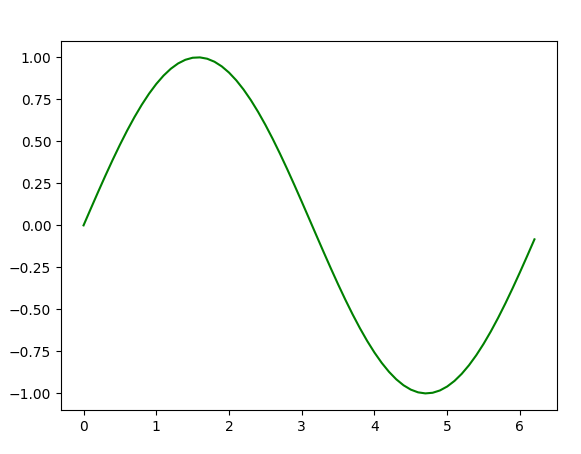
Here, we use NumPy which is a general-purpose array-processing package in python.
- To set the x-axis values, we use the np.arange() method in which the first two arguments are for range and the third one for step-wise increment. The result is a NumPy array.
- To get corresponding y-axis values, we simply use the predefined np.sin() method on the NumPy array.
- Finally, we plot the points by passing x and y arrays to the plt.plot() function.
So, in this part, we discussed various types of plots we can create in matplotlib. There are more plots that haven’t been covered but the most significant ones are discussed here –
This article is contributed by Nikhil Kumar. If you like GeeksforGeeks and would like to contribute, you can also write an article using write.geeksforgeeks.org or mail your article to [email protected]. See your article appearing on the GeeksforGeeks main page and help other Geeks.
Please write comments if you find anything incorrect, or you want to share more information about the topic discussed above.
Also Read: What are the combinational logic circuits?