How to Make Histograms with Density Plots with Seaborn histplot? In this instructional exercise, we will perceive how to make a histogram with a thickness line involving Seaborn in Python. With Seaborn rendition 0.11.0, we have another capacity histplot() to make histograms.
Here, we will figure out how to utilize Seaborn’s histplot() to make a histogram with thickness line first and afterward perceive how to make various covering histograms with thickness lines.
Histograms are representation instruments that address the appropriation of a bunch of constant information. In a histogram, the information is isolated into a bunch of stretches or canisters (ordinarily on the x-pivot) and the count of information focuses that fall into each container comparing to the tallness of the bar over that receptacle. These canisters could possibly be equivalent in width yet are adjoining (without any holes).
A thickness plot (otherwise called part thickness plot) is another perception device for assessing information dispersions. It tends to be considered as a smoothed histogram. The pinnacles of a thickness plot assist with showing where esteems are concentrated over the span. There are an assortment of smoothing methods. Piece Density Estimation (KDE) is one of the procedures used to smooth a histogram.
How to Make Histograms with Density Plots with Seaborn histplot?
Seaborn is an information representation library in view of matplotlib in Python. In this article, we will utilize seaborn.histplot() to plot a histogram with a thickness plot.
Grammar: seaborn.histplot(data, x, y, tint, detail, receptacles, binwidth, discrete, kde, log_scale)
Boundaries:
- Information: input information as Dataframe or Numpy cluster
- X, Y (discretionary): key of the information to be situated on the x and y tomahawks individually
- Shade (discretionary): semantic information key which is planned to decide the shade of plot components
- Detail (discretionary): count, recurrence, thickness or likelihood
- Return: This technique returns the matplotlib tomahawks with the plot drawn on it.
Example 1:
- Python3
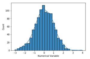
# Import necessary librariesimport seaborn as snsimport numpy as npimport pandas as pd# Generating dataset of random numbersnp.random.seed(1)num_var = np.random.randn(1000)num_var = pd.Series(num_var, name = "Numerical Variable")# Plot histogramsns.histplot(data = num_var, kde = True) |
Output:
Example 2:
- Python3
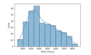
# Import necessary librariesimport numpy as npimport pandas as pdimport seaborn as sns# Load datasetpenguins = sns.load_dataset("penguins")# Plot histogramsns.histplot(data = penguins, x = "body_mass_g", kde = True) |
Output:
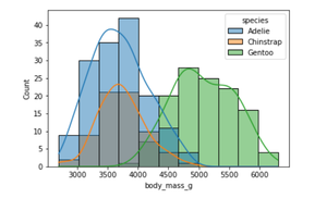
We can also visualize the distribution of body mass for multiple species in a single plot. The hue parameter maps the semantic variable ‘species’.
- Python3
# Plot Histogramsns.histplot(data = penguins, x = "body_mass_g", kde = True, hue = "species") |
Output:
Example 3:
- Python3
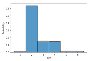
# Import necessary librariesimport numpy as npimport pandas as pdimport seaborn as sns# Load datasettips = sns.load_dataset("tips")# Plot histogramsns.histplot(data = tips, x = "size", stat = "probability", discrete = True) |
Output:
Also Read: Returning Multiple values in Java