Gram Schmidt Orth-normalization Based Projection Depth. GSO (Gram-Schmidt Orth normalization) is based on depth function of Euclidean vector which can be proposed to compute the projection depth. The performance of GSO can be studied to exact and approximate algorithms, bivariate data (data from two variables) can be used to associate estimation namely Stahel-Donoho (S-D) location and scatter estimation. The efficiency can be checked by computing average misclassification error in discriminant analysis under real and stimulating environment. The study about GSO can be concluded that the estimators only perform well when it will be compared with exact and approximate algorithms.

INTRODUCTION:

Data depth is a function which is situated in the centrality of a given point data cloud. It is closely related to central regions of a data cloud. It plays an important role in many field of statistics, namely used; data exploration, ordering, asymptotic distributions and robust estimation. The main idea is that, a central point is located in a multiple variant of data cloud only if it is located centrally in each single variant projection of this data cloud. The depth of a point in a multiple variant data cloud is defined as the minimum of the depth arising from the single variant projection of the data.

This paper tells us about projection depth and associate estimator. The computation represent the algorithm namely Gram Schmidt Orth normalization. This process also examines the GSO algorithm and various algorithm projection depths.

EXPLANATION:

PROJECTION DEPTH AND ITS ASSOCIATED ESTIMATOR:

Create a projection-based depth function, which has the highest breakdown point among all the existing characterized equal variant multivariate location estimators and associated medians. The projection depth is appeared very favorable to robust statistics when compared with the others depth notions. It is due to all the desirable properties of the general statistical depth function defined in namely, characterized invariance, maximally at center, monotonicity relative to deepest point, and disappear at infinity are satisfied. Also, it can induce the favorable estimators, such as Stahel-Donoho estimator and depth weighted means for multivariate data. Introduced the concept of multidimensional cuttings on projection depth. Exact computation of bivariate projection depth and Stahel-Donoho estimator, furthermore, with a proper choices of (µ, σ) are formulated and studied by. Further computing issues of projection depth and its associated estimators have studied by. The basic idea of computing, projection depth is summarized given below.

Let µ (.) and σ (.) be univariate location and scale measures, respectively. Then the outlining of a point xÎR^P with respect to distribution functions F of X is denoted by given formula.

O( x,F )=sup | Q(u,x,F ) ||u||^-1

Q(x,F )=(u^Tx-µ(Fn))/σ(Fu)

Fu is the distribution of u^T x. If u^Tx-µ(Fu) =σ(Fu)=0, and Q(u,x,F) = 0 , which denotes the projection of x onto the unit vectors u. Note that the most popular outlying whereas the µ is the median (med) and σ is the median absolute deviation (MAD). And it is denoted by (med,MAD) and Q(x,u,X^n).

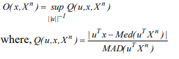
Where u^T denotes the projection of x in unit vector u

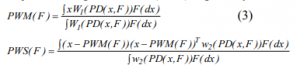
Other formula of the famous Stahel-Donoho location estimator is the Projection Weighted Mean (PWM) and Projection Weighted Scatter (PWS) is given by

GSO PROCEDURE OF COMPUTING PROJECTION DEPTH:

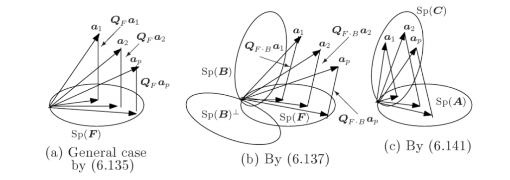
As we know that the orthonormal factor can be finding by gram Schmidt process. First of all find the orthogonal factor with their respective vectors. The fixed direction procedure uses fixed m directions which cut the upper half plane equally, and chooses the direction which can maximize. While random direction procedure randomly picks some m directions and chooses the optimal direction for computing the projection depth. The detailed computational steps are given by. An exact algorithm of computation of bivariate projection depth and the Stahel-Donoho estimator has been studied by. Further, the simplified version of the computational procedure is given by

In mathematics, particularly linear algebra and numerical analysis, the Gram-Schmidt process is a method for orthogonal normalization of vectors in an inner product space, most commonly the Euclidean space Rn equipped with the standard inner product. The Gram-Schmidt process takes a finite, linearly independent set {v1,…,vk} for k £ n and generates an orthogonal set {v1,…, vk} that spans the same k dimensional subspace of Rn as S. The basic idea of Gram-Schmidt process is as follows: Let u1 = v1 that is

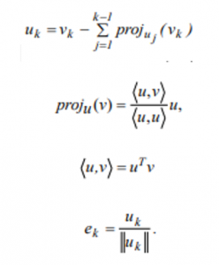
Is the orthogonal vectors, and the normalized vectors e1,…,ek form an orthonormal set. The computation of the sequence u1,…,uk is known as Gram-Schmidt orthogonalization, while the computation of the sequence e1,…,ek is known as Gram-Schmidt orthonormalization as the vectors are normalized. When this process is implemented on the vectors 𝑢𝑘 are often not quite orthogonal, due to rounding errors. The Gram-Schmidt process can be stabilized by a small modification. Instead of computing the vector 𝑢𝑘 as in, it is computed as

NUMERICAL ANALYSIS:

To illustrate the performance of projection depth, a real data example is presented. The data set is taken from (Sweat data, Page 215). The data consists of 19 observations. The data describe 19 healthy females were measured with two variables sweat rate (X1) and sodium content (X2). The projection depth-size plots are displayed in the figure. It is noted that the larger size of the dot corresponds to the larger depth of the point. The computed projection depth values under the various algorithms with GSO are presented

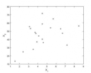
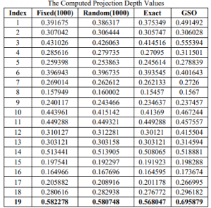
It is noted that the 19th observation is the largest data occur in it and the larger depth value. Further comparing the depth value under various algorithms, the GSO gives the highest among them.

SIMULATION RESULT:

A simulation study is performed to compare the efficiency of the proposed GSO procedure along with various notions of projection depth procedure. The data (n=25) are generated from a multivariate normal distribution, mean vector µ= (0, 0) and the unit covariance matrix, S=I2. The results are listed in table

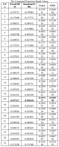
The table indicates that, 17th observation represents the location of generating data, since it has the largest depth value. Further, it is noted that GSO gives the highest depth value compared to the exact and approximate algorithms.

APPLICATION:

The superiority of the GSO over all other algorithm is performing classification techniques computational algorithm is fast for amplification.  Just like Stahel -Donohoe algorithm which is used for the calculating the location and the scatter values, actually it is based on the project depth approach.

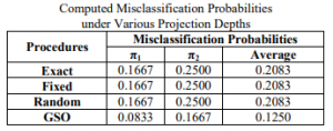
REAL DATA:

The real data is actually consist of two types π one which is riding mower owner and π two with no owner. On these variables incoming x1 and lot size x2. When compared to approximate and exact algorithms, the GSO algorithm produces a substantially lower misclassification rate. That GSO Only 12% of processes is mislabeled, but all others are. Around 21% of the original data is categorized incorrectly.

SIMULATION RESULT:

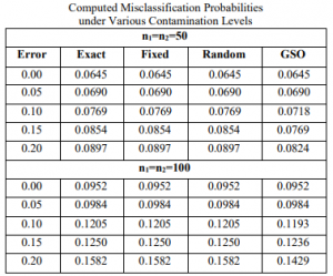
A simulation study with and without contamination is also conducted to compare the GSO process to the approximate and accurate techniques. The data came from two distinct normal distributions (g=2, p=2) with sample sizes ranging from 50 to 100. The data were extracted from a normal distribution with covariance matrices of 1=I2 and 2= 1.5I2, along with means of 1= (1, 1) and 2= (3, 3). The location and scale contaminations are applied as mentioned using the covariance matrices 1 = 3 I2 and 2 = 2I2 and the values of 1= (-4, -4) and 2= (-5, 5) respectively. In two situations, different amounts of contamination were evaluated, namely 0%, 5%, 10%, 15%, and 20%.It should be highlighted that as the amount of contamination climbs, so do the chances of misclassification under all techniques. When the average likelihood of misclassification values in the above table are compared to the precise and approximate methods, it is clear that the GSO algorithm generates less. The GSO surpasses the absolute and estimate algorithms, according to the results. It indicates that it outperforms the other algorithms with and without contaminated data.

 

CONCLUSION:

This paper presents a novel idea of computing, projection depth. The computational aspect of the GSO algorithm is described. The performance of the GSO algorithm is discussed through numerical analysis. Further, the superiority of the GSO is demonstrated over the exact and approximate procedures by applying it in discriminant analysis under with/without contamination. It is concluded that, the performance of GSO procedure is much better than approximate and exact algorithms. The study can be extended to higher dimensions. The new GSO procedure can be applied in almost all multivariate analysis and in turn it is very useful to research communities doing research in the field of data mining and computer vision.

Also read

What are the Orthogonal and Orthonormal vectors?