Implementation and design of nickel coating thickness tester
Implementation and design of nickel coating thickness tester. “Non Magnetic Coating, Ferrous Base, Thickness Measuring Gauge” works on the principle of Magnetic Induction. Magnetic induction instruments use a permanent magnet as the source of the magnetic field. A Hall-effect generator or magneto-resistor is used to sense the magnetic flux density at a pole of the magnet, which correspondingly produces analog voltage as an output. This analog voltage will be applied as the input to a microcontroller, which in return will show the coating thickness on the display.
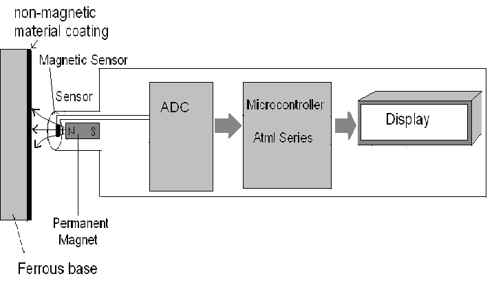
Block Diagram:
The main design of coating thickness gauge is shown in diagram given below :
Modules
We can divide the working of this gauge in four modules:
- Sensor
- ADC(Analog to Digital Converter)
- Microcontroller
- Display
Sensor
Sensor consists of:
- Permanent magnet
- Magnetic field sensor
Permanent Magnet:
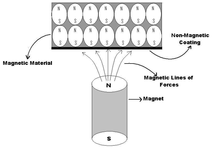
Magnetic field is generated from the permanent magnet. Magnetic lines of forces or magnetic field will become aligned in the presence of ferrous placed in front of it. This magnetic field intensity will be inversely proportional with the thickness of the non magnetic coated material over iron. While there are an infinite number of applications for permanent magnets, they can be classified into four general groups:
Conversion of Electrical Energy to Physical Motion
Examples include motors, actuators, speakers, meters and instruments. In these applications, electrical input causes a relative movement of the magnet which results in the desired physical output.
Conversion of Physical Motion to Electrical Energy
Generators, microphones and sensors are the most common applications for converting physical motion into electrical energy. Relative movement of the magnet produces an electrical output.
Production of Mechanical Energy
In these applications, magnets are used to hold, lift, create tension or apply a repulsive force. Examples include latches, bases and clamps, torque couplings, locking and unlocking devices and separators.
Applied Fields
In these applications, the magnetic field is used in a special way. Often, it is used to control, shape or direct an object or substance. Applications include annealing and plating dipoles, beam control and focusing, spectrometers, plasma positioning and control devices.
The magnet we are using fit in the category of “Conversion of Physical Motion to Electrical Energy”.
What are the Fundamentals of Magnetism?
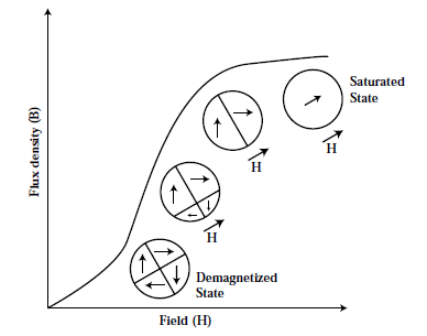
All ferromagnetic materials have atomic magnetic moments that are aligned parallel to each other within small regions called domains. Within these domains, the spontaneous magnetization present is equal to the saturation magnetization of the material, and so the individual domains are fully magnetized at all times. In the absence of an applied field, there is no net magnetic moment or field generated by the material because the magnetization direction of each domain is randomly oriented. During magnetization of the material, domains whose magnetization directions have a component in the direction of the applied field will grow at the expense of those that do not. Once all of the unfavorably oriented domains have been eliminated by domain wall movement, the magnetization direction of the single domain that remains will be rotated to be parallel to of the applied field.
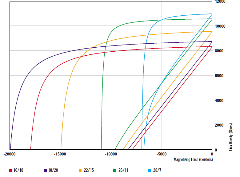
What is Hysteresis Loop?
During magnetization, an increasing magnetic field is applied to the material until a saturation point is reached. Upon removing this applied field, a permanent magnet material will not follow the same path down to flux density = 0, instead, it will retain some of its magnetism. The path that the permanent magnet follows is called a hysteresis loop and is a key tool in the quantitative analysis of permanent magnet performance.
These loops are a graphical representation of the relationship between an applied magnetic field and the resulting induced magnetization within a material. The field that is generated by the now magnetized material (Bi) when added to that of the applied field (H) is known as the normal induction (Bn) or simply B. Since this induction has two components, it is defined as:
B = Bi + H
The B vs H curve is known as the normal curve, while the Bi vs H curve is called the intrinsic curve. Examples of these curves, also known as hysteresis loops, are shown in figure 3.3. The loops show the properties of the magnetic material as it is magnetized and demagnetized.
The second quadrant of the loops displays the magnetic properties as the magnet performs work. By comparing the second quadrant to known parameters within a given magnetic circuit, an approximation of the magnetic output can be determined. When a magnetic field is applied to unmagnetized magnetic material, the intrinsic induction (Bi) is established
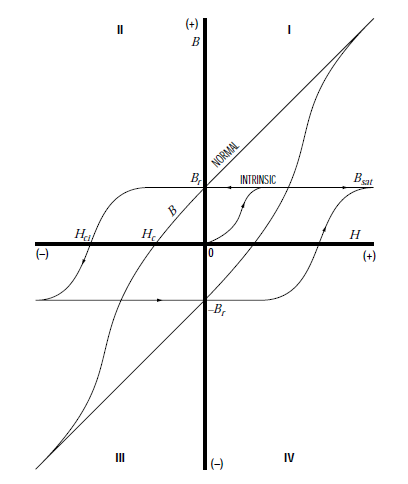
within it, parallel to the applied field. If H is sufficiently strong, the magnet will become fully magnetized at the saturation flux density (Bsat). When the field is reduced to zero, the magnet will recoil to the residual value or remanence (Br), as long as the magnet is within a closed magnetic circuit. Unlike soft magnetic material, the absence of an external magnetic field does not lead to demagnetization. One or more air gaps introduced into a magnetic circuit will enable useful work to be performed.
The mechanical energy used to separate a magnet from soft iron is stored as potential energy within the air gap and the magnet. This moves the point of operation on the intrinsic curve to the second quadrant. The normal curve in the second quadrant represents the energy output of the magnet and is used during magnet design. If the iron in the circuit is completely removed, the air gap becomes very large and the operating point of the curve now approaches Hc in the second quadrant (known as normal coercivity) and the induction (B) will approach zero.
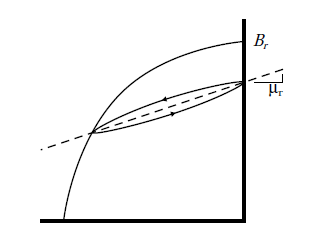
If the air gap is closed again, the stored potential energy is used to perform the work of bringing the magnet and the iron together. The operating point does not, however, return to Br. The magnet recoils along a so-called minor hysteresis loop to a point below Br Repeated opening and closing of the air gap will result in the magnet cycling along this minor hysteresis loop.
The average slope of the minor loop is the recoil permeability (μr).If the demagnetizing field is increased beyond Hc , the operating point of the magnet now moves into the third quadrant of the normal curve. Ultimately, when the intrinsic coercivity (Hci) is reached, the magnet is completely demagnetized. This value is a measure of the magnet’s ability to resist demagnetization.
Materials
There are four major families of permanent magnet materials commercially available. They range from ferrite, which is low cost and low energy to rare earth materials, which are high cost and high energy. Many factors affect the choice of magnetic material, such as operating temperature, size and weight constraints, environmental concerns and required magnetic energy. Each family of materials has several grades with a range of magnetic properties.
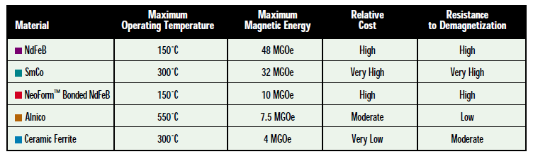
Alnico:
Alnico was developed and made commercially available in the 1940’s. It is an alloy of aluminum, nickel, cobalt and iron. Different grades of Alnico also contain other elements to enhance the magnetic properties. Alnico magnets are generally formed by casting molten alloy or pressing and sintering a very fine powder.
Both forms can be cut and ground to precision sizes with the proper equipment. Energy products for Alnico materials range from 1.5 to 7.5 MGOe. Alnico has the lowest resistance to demagnetization, but the best resistance to temperature effects of all the magnetic materials. Alnico can be used in environments up to 550°C (1020°F) and also in applications where stability is needed across wide temperature ranges.
Discuss Eight Magnetic Axioms?
- Flux lines, like electrical currents, will always follow the path of least resistance. In magnetic terms, this means that flux lines will follow the path of greatest permeance (lowest reluctance).
- Flux lines repel each other if their direction of flow is the same.
- As a corollary to condition two [2], flux lines can never cross.
- As a corollary to condition one [1], flux lines will always follow the shortest path through any medium. They therefore can only travel in straight lines or curved paths, and they can never take true right-angle turns. Meeting the terms of condition two [2], flux lines will normally move in curved paths; although over short distances, they may be considered straight for practical purposes.
- For unsaturated ferromagnetic materials, flux lines will always leave and enter at right angles.
- All ferromagnetic materials have a “limited ability” to carry flux. When they reach this limit, they are saturated and behave as though they do not exist (like air, aluminum and so on). Below the level of saturation, a ferromagnetic material will substantially contain the flux lines passing through it. As saturation is approached, because of conditions one [1] and two [2], the flux lines may travel as readily through the air as through the material.
- Flux lines will always travel from the nearest north pole to the nearest south pole in a path that forms a closed loop. They need not travel to their own opposite pole; although they ultimately do if poles of another magnet are closer and/or there is a path of lower reluctance (greater permeance) between them.
- Magnetic poles are not unit poles. In a magnetic circuit, any two points equidistant from the neutral axis function as poles, so that flux will flow between them (assuring that they meet the other conditions stated above).
Our gauge works on the 7th principle from eight magnetic axioms. The south pole created by dipole moment of atoms of magnetic material placed in front of magnet are more close to the magnet as compared to its own south pole which cause magnetic lines of forces to aligned with respect to that magnetic material. This magnetic field intensity will be measured by sensor as shown in fig.
Magnetic Field Sensor:
The Hall effect was discovered by Dr. Edwin Hall in 1879. Dr. Hall found when a magnet was placed so that its field was perpendicular to one face of a thin rectangle of gold through which current was flowing, a difference in potential appeared at the opposite edges. He found that this voltage was proportional to the current flowing through the conductor, and the flux density or magnetic induction perpendicular to the conductor. Although Hall’s experiments were successful and well received at the time, no applications outside of the realm of theoretical physics were found for over 70 years.
Theory of the Hall Effect
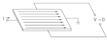
When a current-carrying conductor is placed into a magnetic field, a voltage will be generated perpendicular to both the current and the field. This principle is known as the Hall effect. Following Figure illustrates the basic principle of the Hall effect. It shows a thin sheet of semi conducting material (Hall element) through which a current is passed.
The output connections are perpendicular to the direction of current. When no magnetic field is present current distribution is uniform and no potential difference is seen across the output. When a perpendicular magnetic field is present, as shown in Figure below, a Lorentz force is exerted on the current. This force disturbs the current distribution, resulting in a potential difference (voltage) across the output. This voltage is the Hall voltage (VH). The interaction of the magnetic field and the current is shown in equation below
VH α I × B
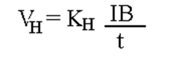
Where I is in amperes, B is in gauss and t is in centimeters. The proportionality constant is called the Hall Coefficient and has the units of volt-cm per ampere gauss. Typical values of Kh for several materials are given in table:
Properties of different conductors used in Hall-Effect Magnetic Field Sensor
| Material | Field Strength, G | Temp. , oC | KH |
| AS | 4,000-8,000 | 20 | 4.52×10⁻¹¹ |
| C | 4,000-11,000 | Room | -1.73×10⁻¹⁰ |
| Bi | 1,130 | 20 | -1×10⁻⁸ |
| Cu | 8000-22,000 | 20 | -5.2×10⁻¹³ |
| Fe | 17,000 | 22 | 1.1×10⁻¹¹ |
| n-Ge | 100-8,000 | 25 | -8×10⁻⁵ |
| Si | 20,000 | 23 | 4.1×10⁻⁸ |
| Sn | 4000 | Room | -2×10-14 |
| Te | 3000-9000 | 20 | 5.3×10⁻⁷ |
Analog output sensors
The sensor described in Figure is a basic analog output device. Analog sensors provide an output voltage that is proportional to the magnetic field to which it is exposed. Although this is a complete device, additional circuit functions were added to simplify the application. The sensed magnetic field can be either positive or negative. As a result, the output of the amplifier will be driven either positive or negative, thus requiring both plus and minus power supplies. To avoid the requirement for two power supplies, a fixed offset or bias is introduced into the differential amplifier. The bias value appears on the output when no magnetic field is present and is referred to as a null voltage. When a positive magnetic field is sensed, the output increases above the null voltage.
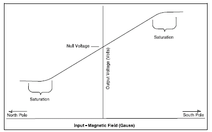
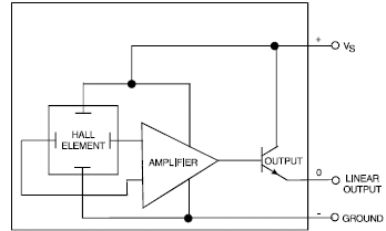
Conversely, when a negative magnetic field is sensed, the output decreases below the null voltage, but remains positive. This concept is illustrated in Figure above. The output of the amplifier cannot exceed the limits imposed by the power supply. In fact, the amplifier will begin to saturate before the limits of the power supply are reached. This saturation is illustrated in Figure It is important to note that this saturation takes place in the amplifier and not in the Hall element. Thus, large magnetic fields will not damage the Hall effect sensors, but rather drive them into saturation. To further increase the interface flexibility of the device, an open emitter, open collector, or push-pull transistor is added to the output of the differential amplifier. Figure shows a complete analog output Hall effect sensor incorporating all of the previously discussed circuit functions.
Also read here