
Introduction
Power Method and Inverse Power Method for Eigen Values and Eigen Vectors. When looking for the greatest Eigen-pair, the power approach is usually used. The Inverse Power approach, on the other hand, is used to determine the smallest Eigen-pair. Other desired Eigen pairs can be found using the shifting property, the Power method, and/or the Inverse Power method. Here are several lemmas based on the Power technique with shifting property.
Furthermore, a Modified Hybrid Iterative Algorithm based on both the Power and Inverse Power methods is proposed to easily find both the largest and smallest Eigen-pairs. Several experiments were carried out to test the algorithm’s robustness and effectiveness. The suggested technique can successfully and efficiently locate both (biggest and smallest) Eigen-pairs. Furthermore, the suggested method is capable of determining the nature (positive and negative sign). In some circumstances, the technique can also determine the second greatest Eigen pair as a result of the Eigen values.
There are some efficient approaches in the literature that are specialized to determining solely Eigen values. However, much more effort is needed to find matching Eigen vectors. The QR-algorithm, which can find all Eigen values, is the most well-known direct technique. This method is based on the QR decomposition of the matrix and is also implemented in software packages such as the Matlab function eig ().
The QR iterative algorithm for calculating the Eigen values of a general matrix was proposed by Heinzultisha user in 1958 and derives from the elegant and simple idea refined by Francis from 1961 to 1962. However, this method does not find the corresponding eigenvector. On the other hand, Power method for Eigen value problems is implemented in various fields of application where only largest Eigen pairs are important. Again Inverse Power method is used to find out smallest Eigen pair.
Moreover, using shifting property, Power method and/or Inverse Power method is also applicable to find out desired Eigen pair. It is important to note that various areas of science and engineering seek both largest as well as smallest Eigen pairs for different reasons other than algorithmic gains. There exist some important fields of application in which second largest (smallest) Eigen pair are also required.
Beside Power method and Inverse Power method, there are several methods available which are able to find both Eigen values and Eigen vectors. Chang et al. proposed several refinements of the Power method that enable the computation of multiple extreme Eigen pairs of very large matrices by using Monte Carlo simulation method.
Panju examined some numerical iterative methods for computing the Eigen values and Eigen vectors of real matrices. He examined five methods – from the simple Power iteration method to the more complicated QR iteration method. The derivations, procedure, and advantages of each method are briefly discussed there.
Besides, Zhang P. et al. have recently developed a general solution strategy for Power method. Recently, Li et al. propose a bound for ratio of the largest Eigen value and second largest Eigen value in module for a higher order tensor.
From this bound, one may deduce the bound of the second largest Eigen value in module for a positive tensor, and the bound can reduce to the matrix cases. In, a general solution strategy of the modified power iteration method for calculating higher Eigen modes has been developed and applied in continuous energy Monte Carlo simulation. A variant of power method is applied to continuous energy.
Preliminaries
Before presenting the proposed algorithm, it is worth discussing some related issues. If A is a square matrix, the matrix Eigen value problem is defined as:
Ax = λx (1)
Where λ is called the Eigen value, x (≠ 0) is the corresponding eigenvector, that is, (λ, x) is called the Eigen pair.
It should be noted that the power method can find the maximum Eigen value, which is referred to herein as the first Eigen value. The power method, on the other hand, allows you to find more Eigen values by using the displacement property. If the shifted parameter is the first Eigen value, then this shifted Eigen value is called the second Eigen value. Incorporating these two terms yields the following characteristics and results (Lemma 1-4):
Property (first Eigen value): The Eigen value obtained by the power method is the largest of all Eigen values, but it is not always the largest in the actual value. Properties (shift properties): If (λ, x) is any Eigen value of equation (1) and α is any scalar quantity, then (λα) is the Eigen value of (A − al). So we have
(A − al) x = (l − a) x (2)
Where (λα, x) is the Eigen pair of the sliding Eigen value problem (2).
Property (second Eigen value): By shifting the property and shifting by the first (maximum) Eigen value, the method to be modified can find another Eigen value and the corresponding eigenvector. Using these properties in the power method, Jamali and Alam [9] proposed some lemmas shown below.
Lemma 1: If the first (maximum) Eigen value is positive and the second Eigen value is also positive (generated by shifting the maximum value), the first Eigen value is maximum in both magnitude and actual value. The second Eigen value, on the other hand, is the smallest in terms of both quantity and value. Therefore, all Eigen values have a positive sign.
Lemma 2: If the first (maximum) Eigen value is positive and the second Eigen value is negative (created by shifting the maximum value), the first Eigen value is maximum in both magnitude and actual value. The second Eigen value (obtained by the algorithm), on the other hand, is the actual minimum, but the largest of all negative Eigen values (if any). As a result, some Eigen values are positive with the largest Eigen value, and some Eigen values have a negative sign (if any).
Lemma 3: If the first (maximum) Eigen value is negative and the second Eigen value is also negative (created by shifting the maximum value), the first Eigen value is maximum, but the actual value is minimum. The second Eigen value, on the other hand, is the smallest in absolute value, but the largest in actual value. As a result, all Eigen values have a negative sign.
Lemma 4: If the first (maximum) Eigen value is negative and the second Eigen value is positive (generated by shifting the maximum value), the first Eigen value is maximum, but the actual value is minimum. The second Eigen value, on the other hand, is the largest actual value and is also the largest of all positive Eigen values (if any). As a result, some Eigen values have a negative sign with the largest Eigen value, and some Eigen values have a positive sign (if any).
See our paper [9] for evidence and extensive discussion. In the next section, we have developed a modified hybrid iteration algorithm based on these lemmas. In fact, the proposed approach is an algorithm that uses the power method and the inverse power method as needed. These lemmas implicitly control the execution flow of the proposed algorithm. In addition, it helps to clearly identify the nature of the Eigen values.
Proposed Modified Hybrid Iterative Algorithm
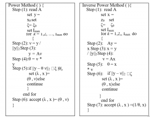
Since the proposed algorithm is based on both the power method and the inverse power method, it is important to briefly review the algorithms of these two methods [see Tables 1 and 2]. Note that using displacement properties, due to the nature of the Eigen spectrum, it may not be possible to find the absolute smallest Eigen pair by the power method. In this situation, the
inverse method is needed to find the smallest Eigen pair.
Using the lemma, we have developed a hybrid modified iteration (HMI) algorithm that detects the properties of both maximum and minimum Eigen pairs and Eigen spectral cans by hybridizing both the power and inverse power methods. The proposed HMI algorithm is shown below:
Modified Hybrid Iterative Algorithm ( )
{
Step (1): read A
Set B=A
Set{λ, x}={λ0, x0} for r =1, 2 do
{
if r =1
{
Step (2): apply Power method ( )
output {λ1, x1}
Step (3) : find s1, such that λ1 =s1|.?1| Step (4): output {λ1, x1, s1}
r = r+1
}
else if r =2
{
Step (5): set B=A– λ1I
Step (6): apply Power method ( )
output {σ2, y2}
Step (7) : λ2 = σ2+ λ1
find s2, such that λ2 = s2|.?2| Step (8): output {λ2, x2, s2}
}
}
end for
Step (9) : if (s1 = s2 and > 0)
{
Output :
{(λ1, x1), (λ2, x2),(all λi≥ 0)} Step (10) : Stop
}
else if (s1= s2 and <0)
{
Output :
{(λ1, x1), (λ2, x2),(all
λi≤ 0)} Step (11) :
Stop
}
else if (s1≠ s2 and s1> 0)
{
Output : {(λ1, x1), (λ2, x2),(sign of all λi
)} Step (12) : continue
}
else if (s1≠ s2 and s1<0)
{
Output : {(λ1, x1), (λ2, x2),( sign of all λi)} Step (13) : continue
}
Step (14) : Set B =A
Set{λ, x}={λ0, x0}
Step (15) :Apply Inverse Power method ( )
output f.?∗ , x3}
3
Step (16) : find s3, such that .?∗ = s3|.?∗ |
3 3
Step (17): Output :3{(λ1, x1), (.?∗ , x3),( sign of all λi)} Stop (18):Stop and end
}
The proposed MHI algorithm is able to find out both the largest and the smallest Eigen pairs, and the nature of Eigen spectrums. Moreover, in some cases the algorithm is also able to find out second smallest Eigen pairs successfully.
In the pseudo code of the proposed algorithm, we have observed that there is a for loop, with index r = 1 and 2, which is analogous to Power method. The first larger loop will start with r =1. When r =1, for the call of function Power method ( ), the algorithm will be able to produce largest Eigen pair. In step (4), the algorithm determines the sign of the maximum Eigen value.
This helps identify the second Eigen value. After performing step (4), increase the value of r to 2. Therefore, on the second iteration in this loop, the algorithm skips from step (2) to step (4), and as a result, the algorithm starts execution from step (5). In step (5), the original matrix A is converted to B by the shift element λ1, so the Eigen values are the bare Eigen values of A, but they are shifted by λ1 (the maximum Eigen value of A).
Again, the algorithm calls the Power method () function. Therefore, again the function Power method( ) produces the largest Eigen pair of B rather than A. Consequently, in step (8), the algorithm finds out second Eigen pairs of the given matrix A successfully. As the value of r = 2, the algorithm escape from the first major loop and enter into next step namely Step (9). The Step (9) consists of some conditional arguments.
If the sign of both Eigen values are same then without executing the function Inverse Power method ( ) the algorithm is able to find out both absolutely largest and smallest (ignore the sign) Eigen values, corresponding Eigen vectors and nature of Eigen spectra. However, if both Eigen values do not have the same sign, the second Eigen value generated by the power method () is not the absolute (unsigned) minimum Eigen value, even if it is the smallest.
Therefore, the algorithm goes to the next step. H. Steps (14), (15), (16), (17) and finally (18). When the algorithm performs step (15), the inverse iter () function is executed. As a result, the absolute minimum Eigen value and the corresponding eigenvector are found along with the type of Eigen value.
In order to check the effectiveness of the proposed set of rules and validity of the lemmas simultaneously (because the set of rules carries those lemmas implicitly) we’ve carried out the set of rules and accomplished numerous extensive numerical experiments. At first we’ve accomplished 12 Test Prob. 1and output is experiments on a12 said with inside the Table three. To check the validity of the proposed set of rules and the lemmas, the hassle is likewise solved via way of means of Mat Lab solver and output is likewise included with inside the Table three particularly closing column of the table. It is determined that the proposed set of rules unearths the primary Eigen fee 43.6996and signal of the Eigen fee is
fantastic. On the opposite hand, we’ve additionally determined that the most important Eigen fee received via way of means of the Mat Lab solver is likewise 43.6996. That is the set of rules is effectively capable of discover the most important Eigen fee. Now we take a look at that the second one Eigen fee received via way of means of the set of rules is – 15.8665 and signal of the second one Eigen fee is bad. So in step with the lemma 2, the second one Eigen fee isn’t smallest (in significance) Eigen fee however biggest Eigen fee amongst all of the bad Eigen values. Moreover, the spectrums of Eigen fee encompass each fantastic and bad value wherein the most important fee is of fantastic signal. We take a look at that the experimental effects believe the lemmas. That is the second one Eigen fee isn’t smallest Eigen fee concerning significance however biggest in significance amongst all bad fee eleven though smallest Eigen fee if we remember signal of every Eigen fee. Now seeing that the second one Eigen fee isn’t in reality smallest Eigen fee, so for locating out the smallest (in magnitude).
| Eigen pairs and sign of Eigen value obtained by Modified Hybrid
Iterative Algorithm |
Eigen values (Mat
Lab). |
|||
| Eigen value | Sig n | Eigen values
(.?) |
Eigen
vecto r (X) |
|
| First Eigen | [0.92073, 0.782303, | |||
| Value | 0.851719, | |||
| (Largest Eigen | + ve | 43.6996 | 0.767980, 1.000000, | 43.6996 |
| value ) | 0.876090 , | |||
| ( in magnitude) | 0.849523, 0.453403, | 12.15 | ||
| 0.599790, | 65 | |||
| 0.641932, 0.480074, | 10.80 | |||
| 0.799947] | 18 | |||
| Second Eigen value (second Largest negative
Eigen value (among the negative values) |
[-0.708442,-0.233479, |
7.8891 |
||
| – ve | -0.394794,0.193943, | 5.9091 | ||
| 1.00000, – | ||||
| – | 0.124613,0.721741, | 1.816 | ||
| 15.8665 | 0.195695, | 0 | ||
| 0.801014,0.0019818, | – | |||
| -0.731598, -0.876232] | 0.721 | |||
| 0 | ||||
| – | ||||
| 4.908 | ||||
| 2 | ||||
| Smallest Eigen
value |
– ve |
-0.72098 |
[ 0.10929, -0.261378, | -6.5833 |
| (in magnitude) | -0.274267, 0.241883, | -8.4682 | ||
| -0.106012,0.0853739, | – 0.7250 | |||
| -0.394766, 1.000000,
0.174666, -0.0421989, 0.421505, |
– 15.8666 | |||
| -0.26894] | ||||
| Second smallest | + ve | [ -0.115199 ,0.224341, | ||
| positive | ||||
| Eigen value | -0.00357368, | |||
| 1.81593 | -0.416398 , -0.0414743 | |||
| 7 | ,0.189909, | |||
| 0.21043 , – | ||||
0.408524,0.382283, –
|
The Eigen values and the corresponding eigenvectors, the algorithm needed to perform more steps, and the next subsequent step performed the inverse iter () function. Therefore, the algorithm finds an Eigen value with a value of 0.72098 and a negative sign. The minimum Eigen value obtained by Mat Lab is 0.7210, which is observed to be approximately the same as the Eigen value obtained by the proposed algorithm. Also, make sure that the algorithm can not only find the Eigen values, but also the corresponding eigenvectors. This is shown in column 4 of Table 3. Now, for further experimental investigation, we examined the test sample. Shown below 2. This is observed with a test probability. In FIG. 2, the transformation matrix F is of order 8. The experimental results are shown in Table 4. The results in Table 4 were also compared to compare the proposed algorithm with the results obtained from the Mat Lab solver.
57 37 50 21 25 22 -3 20
37 44 40 28 12 29 27 07
50 40 85 31 40 36 23 22
21 28 431 80 7 18 16 15
25 12 40 07 59 20 15 08
22 29 36 18 20 34 24 10
-3 27 23 16 15 24 11 -3
20 07 02 15 08 10 -3 61
It is observed that the signs of both the first and second Eigen values obtained by the proposed algorithm are positive. Therefore, according to the lemma, the first Eigen value must be the absolute maximum Eigen value and the second Eigen value must be the absolute minimum Eigen value. In addition, according to the lemma, all Eigen values must have a positive sign. By comparing the experimental results with the Mat Lab values, we can conclude that the proposed algorithm can efficiently find the largest and smallest unique pairs and justify the lemma.
Table 4: Finding Eigen pairs and comparison of Eigen values for the Test Prob. 2
| Eigen pairs and sign of Eigen value obtained by Modified
Hybrid Iterative Algorithm |
Mat Lab | |||
| Eig en val ue | Eig en valu es
(.?) |
Sign | Eigen vector (X) | All
Eigen value s |
| 1stEige
n |
229.0 48 |
+ve | [0.905122,0.789705,0.877491,0.
733968,1, |
229.04 77 108.08 00 68.721 5 50.378 |
| value | 646421,0.474731,0.91332,0.668
277] |
|||
| (Large st | ||||
| Eigen | ||||
| value) | ||||
| 2ndEig
en |
2.456 |
+ve | [-0.714502, 1, 0.109971, –
0.100363, 0.257215, |
9
38.009 2 18.029 5
15.27732.4 559 |
| value | -0.540873 ,-0.191723, 0.156506] | |||
| (Small
est |
||||
| Eigen | ||||
| value) |
Conclusion
By using the lemma, we have developed a Hybrid Modified Iterative (HMI) algorithm. This algorithm integrates both the power method and the inverse power method to find both the maximum and minimum unique pairs at the same time. Several experiments were conducted to verify the algorithm and lemma. From the numerical experiments examined here, we can conclude that the proposed algorithm can successfully find both the absolute maximum and minimum Eigen values of and the corresponding eigenvectors. In addition, the algorithm can find the properties of the Eigen spectrum. However, the proposed algorithm has some drawbacks of the power method. That is, it finds the Eigen values when the maximum (minimum) Eigen values are duplicated, and finds the complex Eigen values.
Also read here
- Application of Linear Algebra in Computer Graphics
- What is the application of linear algebra in cryptography?
- what are the row spaces, column spaces and null spaces in Linear Algebra?
- How to solve system of linear equations in Linear Algebra?
- what is the vector space in linear algebra? vector space example
- What is Linear combinations, Linear dependence and Linear Independence?