
Why we need tree structure in graph theory? What is the advantage and what are its applications?
In this article, I have discussed in detail about Breadth First Search Algorithm . Trees are important to the structural understanding of graphs and to the algorithmic of information processing, and they play a central role in the design and analysis of connected networks. In fact, trees are the backbone of optimally connected networks. A main task in information management is deciding how to store data in space-efficient ways that also allow their retrieval and modification to be time-efficient. Tree based structures are often the best way of balancing these competing goals.
For example, the binary-search-tree structure leads to an optimally efficient search algorithm. They also enable efficient insertion and deletion operations.
Decision trees are used in machine learning and optimization problems. They help in making decisions by splitting the data based on certain criteria at each node until a decision or prediction is reached at the leaves.
Similarly, Huffman trees are used in data compression algorithms, such as Huffman coding. These trees represent variable-length codes assigned to different characters, enabling efficient compression of data.
Heap data structures, which can be visualized as a type of tree, are used in sorting algorithms like Heap Sort. Trees provide a structured way to organize and access data efficiently.
So, we can say that tree structures in graph theory provide a natural way to model and represent hierarchical relationships, and their properties make them valuable in various applications ranging from computer science and networking to many decision-making problems.
What is the advantage of traversing the tree in in-order, pre-order and post-order form? Any specific applications?
A systematic visit of each vertex of a tree is called a tree traversal. Traversal in binary trees can be done in different orders: in-order, pre-order, and post-order. Each traversal order has its advantages and is suited to specific applications. Here’s a brief overview of each and their applications:
In-Order Traversal:
Order: Left subtree à Root à Right subtree
Advantages:
Sorted Output: In-order traversal of a binary search tree results in a sorted sequence of elements. This property is useful in searching for elements and printing elements in ascending order.
Expression Evaluation:
In the case of expression trees, an in-order traversal helps to generate the infix expression, which is suitable for human readability. It is useful in evaluating arithmetic expressions.
Pre-Order Traversal:
Order: Root àLeft subtree àRight subtree
Advantages:
Prefix Expression:
Pre-order traversal is useful for generating prefix expressions. It is employed in certain applications of expression parsing and evaluation.
Post-Order Traversal:
Order: Left subtree à Right subtree à Root
Application:
Memory Deallocation: In certain tree-based data structures, post-order traversal is used for freeing up memory occupied by the nodes. It ensures that a node is deleted only after its children have been deleted.
Specific Applications:
Expression Trees: Traversing expression trees in different orders is used in parsing and evaluating mathematical expressions. In-order expressions are human-readable, pre-order and post-order expressions are useful in computer-based evaluation.
Binary Search Trees (BST): In-order traversal of a BST gives elements in sorted order, making it useful for searching and printing elements in sorted order.
Binary Tree Manipulation: Traversal orders are employed in various operations like copying a tree, creating a mirror image of a tree, and freeing up memory.
In summary, the choice of traversal order depends on the specific requirements of the application. Each order provides a different perspective on the structure of the tree, making them suitable for different tasks such as expression evaluation, sorting, and memory management.
Understand breath first search tree traversal by yourself and write its algorithm
Breadth First Search Algorithm
This approach involves traversing a tree by breadth rather than by depth. This algorithm is very useful for exploring all the vertices of a graph. The idea is to start at designated source vertex and then explore the neighbours of the original vertex. Once all of these have been examined, their neighbours are explored. This process repeats until all the vertices of the entire graph have been visited. In this way spanning forest of the input graph can be constructed. In the original graph is connected, the exploration forms a structure called a breadth first search tree.
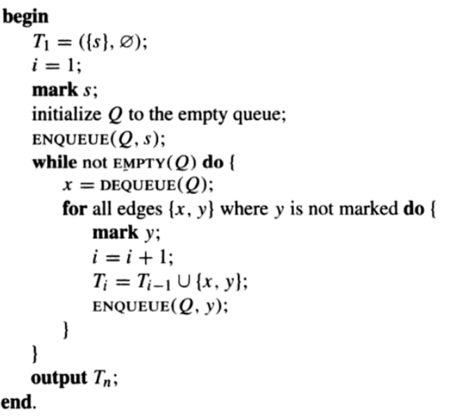
Pseudo code for Breadth First Search (BFS)
Input: A simple undirected graph G (V, E) on n vertices and designated source vertex s.
Output: A breadth First Search Tree
Queue Data Structure
The queue data structure is used for expressing this algorithm. A queue can be thought of as a line such as a grocery store checkout line, where entries are removed from the front, often called the head, and added at the rear, called the tail. An example of the queue is shown below
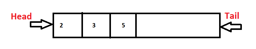
ENQUEUE: Adding an element in the queue at the tail.
DEQUEUE: Removing an element form the head of queue.
EMPTY: Checking to see, if there is anything in the queue.
More formally, the operation ENQUEUE(Q,u) adds u to the tail of Q, thereby increasing the size of Q by one item. The operation DEQUEUE(Q) removes one item form the head of nonempty queue and returns that element. This reduces the queue size by one. The operation EMPTY (Q) returns a value true if the queue has no items and false otherwise.
Breadth-first search is a far better method to use in situations where the tree may have very deep paths, and particularly where the goal node is in a shallower part of the tree. Unfortunately, it does not perform so well where the branching factor of the tree is extremely high, such as when examining game trees for games like Go or Chess.
Breadth-first search is a poor idea in trees where all paths lead to a goal node with similar length paths. In situations such as this, depth-first search would perform far better because it would identify a goal node when it reached the bottom of the first path it examined.
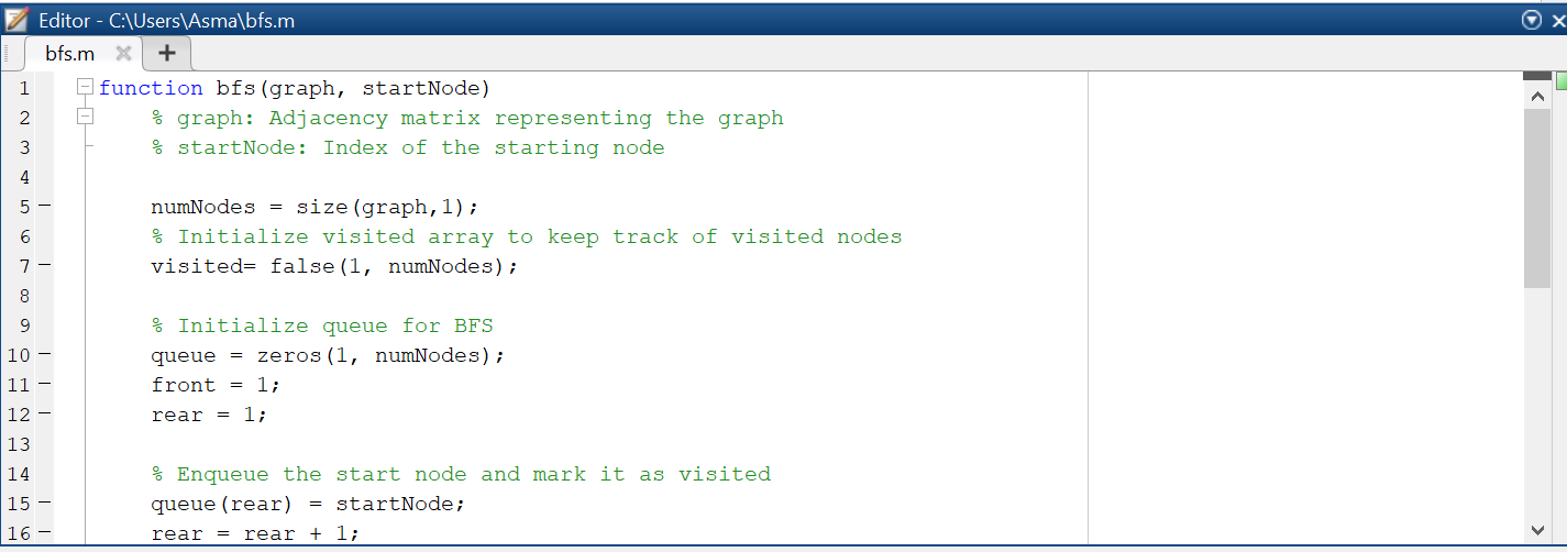
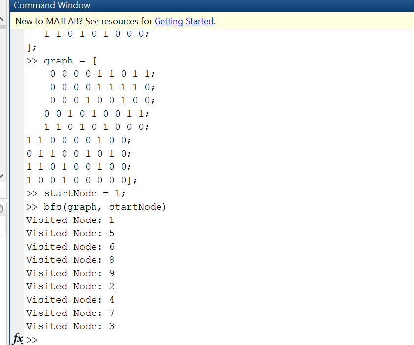
MATLAB Code for Breadth First Search
I have used the adjacency matrix of the above graph for applying the BFS method.
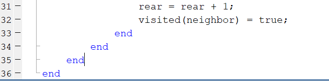
function bfs(graph, startNode)
% graph: Adjacency matrix representing the graph
% startNode: Index of the starting node
numNodes = size(graph,1);
% Initialize visited array to keep track of visited nodes
visited= false(1, numNodes);
% Initialize queue for BFS
queue = zeros(1, numNodes);
front = 1;
rear = 1;
% Enqueue the start node and mark it as visited
queue(rear) = startNode;
rear = rear + 1;
visited(startNode) = true;
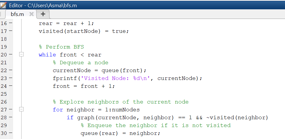
% Perform BFS
while front < rear
% Dequeue a node
currentNode = queue(front);
fprintf(‘Visited Node: %d\n’, currentNode);
front = front + 1;
% Explore neighbors of the current node
for neighbor = 1:numNodes
if graph(currentNode, neighbor) == 1 && ~visited(neighbor)
% Enqueue the neighbor if it is not visited
queue(rear) = neighbor;
rear = rear + 1;
visited(neighbor) = true;
end
end
end
end
Also watch here
Breadth First Search (BFS) Algorithm with Example
In this video lecture I have explained the Breadth First Search Algorithm with an example of the graph. From which I have constructed a Breadth First Search Tree. i have taken an example of 9 nodes. Here it is explained how the Enqueue and dequeue operations are performed in order to construct the tree form the graph until the queue is empty.
Also read here: