Table of Contents

Introduction

The fast Fourier transform method and ill-conditioned matrices. We have studied the problem of calculating numerical solutions of the linear algebra equation, a*x=b, where a denotes an N*N ill-conditioned coefficient matrix. It is known that Gaussian elimination methods linked with swivel arrangements are unproductive in this setting due to round-of error. We intend a new and simple application of the fast Fourier transform (FFT) method. The purpose of this paper is to look into the functionality of the proposed method and compare it to some other methods. The comparison is demonstrated by computer simulation results using MATLAB.

We’ll study the problem of calculating numerical solutions of linear algebraic systems, a*x=b It is well-known that Gaussian elimination linked with swivel arrangements are un useful in this case due to round of error. One can use double precision for better perfection if the hardware permits, however this is not suggested. Or else, we can use various methods programmed to improve the condition number of the coefficient matrix. There have been various methods designed to handle ill-conditioned problems.

Although, some of the methods may involve complicated matrix decompositions with various iteration steps (3±6). The parallel algorithm for Householder transformation has been used for ill-conditioned problems, but we don’t obtain the results valuable. The singular value decomposition method (SVDM) is also a popular method but its tolerance lessens when the calculated eigen values are near zero or zero. So, more adjustment is needed to better the performance of the method.

The Fast Fourier transform (FFT) has been very well used over the last few decades and many computers code has been list to apply the FFT algorithm. The significance of the FFT is that it decreases the number of operations of the discrete Fourier transform (DFT) from O (n ^2) to O (n log2 n). We present a simple and new method that uses the FFT to Fourier transform a and b. Gauss-Jordan reduction is implemented to simplify the resulting linear system and the inverse FFT is implemented to get a numerical solution of the original linear system.

We will develop the algorithm and provide demonstrations using MATLAB simulation. In these simulations, the representation of the FFT method (FFTM) will be compared to the SVDM and QR method. We’ll also use simulations to provide a tolerance test of the FFTM with respect to the dimension of the problem and with respect to the condition number of the coefficient matrix. Finally, we will show that the FFTM is practical for any finite dimensional problem however the FFT is valid only if N is a power of 2. If N is not a power of 2, we use the method of zero-padding so that the FFTM can be employed. In our research, we have gone over 200 experiments. Seldom the coefficient matrix is carefully constructed to show certain desired properties. Seldom the ill-conditioned coefficient matrix has been selected at random. In each case, the FFTM performed better than each of the SVDM and QRM.

Fourier transform properties

The forward and backward Discrete Fourier Transform for any p-periodic function can be described, respectively,

$$
F[k]=\frac{1}{N} \sum_{n=0}^{N-1} f[n] \mathrm{e}^{-2 \pi \mathrm{i} k n / N} \quad(\forall k=0,1,2, \ldots, N-1)
$$
And,
$$
f[n]=\sum_{k=0}^{N-1} F[k] \mathrm{e}^{2 \pi \mathrm{i} k n / N} \quad(\forall n=0, \pm 1, \pm 2, \ldots,)
$$

where f is the given discrete function and n is its variable. F and k are their respective Fourier transforms. N denotes the total number of elements in f. For clarity, we introduce matrix algebra notation. Define the Fourier transform operator as F, where

$$
\mathrm{F}\left[\begin{array}{c}
f[0] \\
\cdot \\
\cdot \\
f[N-1]
\end{array}\right]=\left[\begin{array}{c}
(1 / N) \sum_{n=0}^{N-1} f[n] \mathrm{e}^{-2 \pi \mathrm{i} \cdot 0 \cdot n / N} \\
\cdot \\
\cdot \\
\cdot \\
(1 / N) \sum_{n=0}^{N-1} f[n] \mathrm{e}^{-2 \pi \mathrm{i} \cdot(N-1) \cdot n / N}
\end{array}\right]
$$
Let w be $\mathrm{e}^{\wedge}-2 \mathrm{pi} / \mathrm{N}$. Then $\mathrm{F}$ will have the matrix representation
$$
\mathrm{F}=\frac{1}{N}\left[\begin{array}{cccccccccc}
1 & 1 & 1 & 1 & \cdot & \cdot & \cdot & \cdot & \cdot & 1 \\
1 & \omega & \omega^{2} & \cdot & \cdot & \cdot & \cdot & \cdot & \cdot & \omega^{(N-1)} \\
1 & \omega^{2} & \omega^{4} & \cdot & \cdot & \cdot & \cdot & \cdot & \cdot & \omega^{2(N-1)} \\
\cdot & \cdot & \cdot & \cdot & & & & & & \cdot \\
\cdot & \cdot & \cdot & & \cdot & & & & & \cdot \\
\cdot & \cdot & \cdot & & & \cdot & & & & \cdot \\
\cdot & \cdot & \cdot & & & & \cdot & & & \cdot \\
\cdot & \cdot & \cdot & & & & & \cdot & & \cdot \\
\cdot & \cdot & \cdot & & & & & & \cdot & \cdot \\
1 & \omega^{(N-1)} & \omega^{2(N-1)} & \cdot & \cdot & \cdot & \cdot & \cdot & \cdot & \omega^{(N-1)(N-1)}
\end{array}\right]
$$
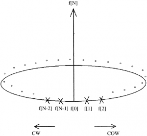
Note that the last and first elements of the function are $\mathrm{f}[0]$ and $\mathrm{f}[\mathrm{N}-1]$, respectively. The dots donate the other remained elements of the function. In the $\mathrm{CW}$ and the $\mathrm{CCW}$ directions, the function can be donated respectively as
$$
f_{\mathrm{CW}}[n]=\{f[0], f[N-1], \ldots, f[2], f[1]\}
$$
And,
$$
f_{\mathrm{CCW}}[n]=\{f[0], f[1], \ldots, f[N-2], f[N-1]\}
$$

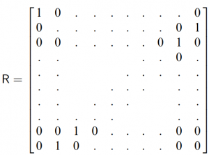
Note that Fccw= R*Fcw is the image of Fcw, where R is the reflection operator. Also, note that the 1st element, f [0] is not shifted after the reflection operation. The reflection operation is represented by the permutation matrix

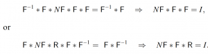
According to the inversion rule of the Discrete Fourier Transform, if g[n] = F [n], then G[k] = N^-1 f [-k], where g and f are two extreme functions and G and F are the respective Fourier transforms. Applying both the Fourier transform and reflection operators and rescript the inversion rule as: if g=Ff, then F g = N^-1 Rf, where f [-k] = Rf [k]. In particular

or F^2 = N ^-1 R. We also note that R * R = R^ 2 = I, where I is identity matrix

Proposed theory

We will 1^st get some identity equations which we given below

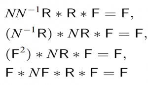
and if we pre multiply or post multiply with F^-1, we obtain

Next, we determine the two-dimensional Discrete Fourier Transform for any N * N coefficient matrix (a). Let A represent the two-D Discrete Fourier Transform of a. A is obtained by performing a one-dimensional Discrete Fourier Transform for every row or for column and led by a 1-D DFT for each column (or row). Most algorithms are written to carry out DFT in one direction, therefore if we perform a 1-D DFT and transpose the result before doing another 1-D DFT and along with another transpose, we can obtain the final result of the 2-D DFT. For the purpose of the discussion, we will spell out the 1-D DFT in the horizontal and the vertical directions as Fx and Fy, respectively. We assume that the software package performs the DFT according to the horizontal direction. That is, Fx = F. So, after the 1^st substitution, Fy = Fx, graphically, we can illustrate the 2-D DFT.

The result is transposed 2^nd time to obtain the final 2D-DFT result. Thus,

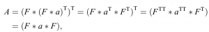
where T is the transpose operation and since F is symmetric, F^T = F. To derive the FFTM algorithm apply the FFT to both sides of the linear system equation to obtain

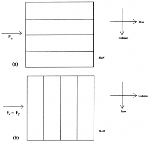
Figure 2Fig. 2. The 1-D DFT (a) in the horizontal direction before the 1^st transpose operation; and (b) in the vertical direction after the 1^st transpose operation.

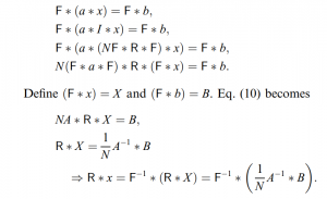
Note that if x = {x [0], …, x [N – 1]}, then R * x = {x [0], x [N – 1] …., x [1]}.

Thus, the solution of the linear system can be calculated by the help of FFTM.

Introduction

Fourier transform properties

Proposed theory

Leave a Reply Cancel reply