Study of Linear Transformation and its Application

In this article you will Study of Linear Transformation and its Application. There were different suspicions and bits of hearsay identified with the idea of direct change which are as following:

This paper is prompting a superior agreement and information about straight change.
Linear transformation obtain inverse (only in the case) if it’s bijective (one-one and onto).
We’ve seen that linear transformations are frequently denoted by matrices. And we’ve number of methods for determining if a matrix is invertible.

Table of Contents

Introduction

Straight change is one of the most special ideas in the direct polynomial math. Various difficulties are observed in a change. Like, a change between registers, especially from the reasonable register to others, Conviction that direct changes should be applied to polygonal things, and accepting the change that saves straight lines is basically straight. The makers suggest that to beat these difficulties, the usage of a powerful estimation environment is required where understudies can see a direct change in three registers (sensible, numerical, and system) simultaneously and as well as the effect of carrying out an improvement in one register on the others.

A part of these difficulties may be related to their late constructed limit originations. Since, a straight change is an unprecedented kind of limit between the vector spaces. By the information gathered, we are analyzing the straight change idea from different focuses. These includes how it is fabricated, what are the related difficulties, originations from the understudies and depictions. The group picked work worldwide brought us to the thought of learning about this idea. The impact of the transformation on the vectors isn’t accessible rapidly. In this specific situation, algorithmic reasoning is overwhelmed. Various responses were encountered to the equal issues in mathematical and arithmetical settings, which assisted understudies by recognizing their errors. Yet, it is not known how much it was useful in building the concept.

Literature Review

Some understudies highlighted the numerical settings, as they are less upheld in the direct polynomial Mathematical courses. In examining some straight polynomial numerical understanding material, like the understudies concludes that it had more troublesome time, finding the recipe of a turn (as it contains mathematical capacities) when chipping away at a displaying issue than with the equation of a shear transformation; in this setting revolution is viewed as more intricate.
Some understudies’ remarks that not all linear transformations conclude a straightforward mathematical understanding, even in the two and three dimensional spaces. However, the models that are related with specific developments in the plane undermine the definition for understudies. Which offered ascend to instinctive models for numerical hypothesis.
These models force certain “results” in the substitute hypothesis. For instance, “a linear transformation does likewise to all vectors.”. An understudy states that, “The instinctive model controls from in the background, the importance, the utilization, the properties of the officially settled concept. The natural model is by all accounts more grounded than the conventional concept“.

Binary Operations

A binary operation is known as a calculation that combines two items to create a new one. A binary operation is also known as a two-arity operation that requires the usage of dual sets of numbers.

Example:

A scalar multiplication of vector spaces produces a vector by taking a scalar and a vector. And, a scalar product produces a scalar by taking two vectors. Instead of using the form f (functional notation) , the binary operations are represented as

In the absence of the operator, powers are written with the second argument superscripted.

Ternary Relation:

The set of triples (a, b, f (a, b)) in S×S×S for any a and b in S given a binary operation f on a set S is called a ternary relation on S.

Linear Transformations

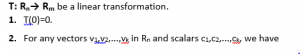
A transformation in which, F: R_n→R_m satisfying the following properties:

linear transformations

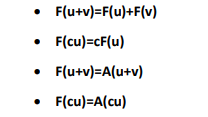
So, A linear transformation is one that satisfies the two defining properties of a matrix transformation.

Multiplication
Addition

The opposite is valid, as any linear transformation is a matrix transformation. Now Let,

Linear transformation properties

Linear Functions (Simple Functions):

That’s why linear functions are accordingly agreeable; in fact, relatively simple functions due to 2 major characteristics:

Linear Transformation with Domain Rⁿ:

A linear transformation with domain R³ is entirely specified by the way it behaves on the three vectors,

vectors

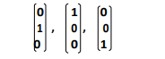
Similarly, the action of a linear transformation with domain Rⁿ on the n distinct n-vectors with exactly one non-zero component completely specifies the transformation, and the matrix from may be retrieved from this information.

Linear Differential Operators

We preferred using the linearity of the derivative operator instead of the limit description of the derivative, studied the power law, as it will be a lot simpler.

Example:

Let T be the vector space of degree either 2 or less having standard addition and scalar multiplication polynomials notated as,

Let, :T → T be the derivative operator. The equations, along with the linearity of the derivative operator, allow to take the derivative of any 2^nd degree polynomial,

polynomial

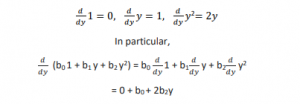
As a result, the derivative of any of the infinite many 2nd order polynomials is determined by just only three inputs.

We see that a linear operator acting on R² is entirely determined by how it acts on the pair of vectors and In fact, any linear operator acting on R2 is also entirely determined by how it acts on and

Example:

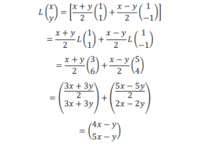
A linear operator L is on the condition called as, when it is entirely specified by two equalities

linear operator

This is since any vector in R² is a sum of multiples of and which can be calculated through a linear systems problems as following:

linear systems problems

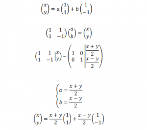
Then, at first representing the vector as a sum of multiples and then putting on the linearity process, one can calculate how L behaves on any sort of vector;

linear problem

As a result, the value of L at just two inputs absolutely defines it. During a similar spirit, there are infinitely many pairs of vectors with the property that each vector in

These types of pair could be called as basis for V. Most likely we have some intuitive notion of what dimension means. Dimension is that the number of independent directions available.

Rank–nullity theorem:-

In linear algebra rank nullity is a theorem, which states that the dimension of the domain of a linear map is that the sum of its rank (the dimension of its image) and its nullity (the dimension of its kernel). Let V,U be a linear vector spaces, where V may be a finite dimensional . rank(T) + Nullity(T) = Dim(V)

here T is that the transformation from V to U. also here:

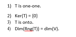
Let V and W be a vector space over F and let Tϵ(V,W). if dim(V) = dim(W) then, the subsequent are equivalent.

Visualizing linear transformation

Algebra of linear transformation: The idea of a transformation can seem more complicated than it really is at first, so before diving into how 2×2 matrices transform two-dimensional space, or how 3×3 matrices transform three dimension space. Let V,W be a vector spaces over F and let S,T ϵ (V,W). Then we define the point-wise Sum of S and T, denoted S + T, by (S+T)(v) = S(v) + T(v), for all v ϵ Scalar multiplication, denoted cT for c ϵ F, by (cT)(v) = c(T(v)), for all v ϵ V.
Equality of linear transformation: Let S,Tϵ (V,W). Then, S and T are said to be equal if S(x) = T(x) . for all xϵV.
Singular and non-singular transformation: Let U and V be a vector spaces over F and let Tϵ(U,V). Then T is said to be singular if 0 ⊊ Ker(T). That is ker(T) is not a zero vector. If Ker(T) is non zero then, T is called non-singular.
Isomorphism of vector space: Let U and V be two vector spaces over F and let Tϵ (U,V), then T is said to be an isomorphism if T is bijective. The vector spaces V and U are said to be isomorphic, denoted U≅ V, if there is an isomorphism from U to V.

Application of Linear Transformation

The geometry of linear transformation in the plane
Reflection in x-axis, y-axis, and y=x
Horizontal and vertical expansion and contraction
Horizontal and vertical shear
Computer graphics(to produce any desire angle of view of a 3-D figure.

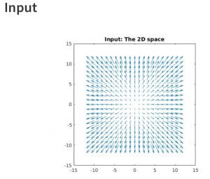
MATLAB Code:

[X Y] = meshgrid(-10:1:10); % coordinates for vector positions

VX = X; % X,Y components of vector

VY = Y;

quiver(X, Y, VX, VY, 2)

title(‘Input: The 2D space’)

axis square

%% reshaping the vectors for linear transformation

YY=reshape(VY,[1 21*21]);

XX=reshape(VX,[1 21*21]);

XY=[XX ;YY];

A=[1 2;-0.5 1]; % Our transformation matrix A

XY_t=A*XY; % linear transform operation

%% This section just creates a “transformed” 2D mesh of vectors

X_t=reshape(XY_t(1,:),[21 21]);

Y_t=reshape(XY_t(2,:),[21 21]);

figure

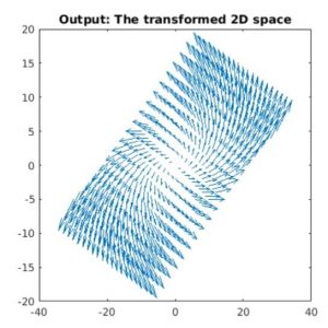
quiver(X_t, Y_t, VX, VY, 2)

axis square

title(‘Output: The transformed 2D space’)

Input and Output:

applications of linear transformations

Conclusion

In this paper we examined about representation and comprehension of direct change. There were different suspicions and bits of hearsay identified with the idea of direct change which are clashed in this paper prompting a superior agreement and information about straight change .A inverse of linear transformation is obtained if and only if it’s bijective (one-one and onto). We’ve also seen that matrices are frequently used to represent linear transformations, and we’ve seen a many methods for determining if a matrix is invertible.

Study of Linear Transformation and its Application

Introduction

Binary Operations

Linear Transformations

Linear Differential Operators

Rank–nullity theorem:-

Visualizing linear transformation

Application of Linear Transformation

Conclusion

Related Topics

Leave a Reply Cancel reply