What is Singular Value Decomposition?

In this article we have discussed about Implementation of SVD ins Machine Learning. SVD, singular value decomposition is one of the methods of dimension reduction. In the field of machine learning, dimension reduction has become an important topic of today in the environment of big data. There are so many methods of dimension reduction but in this paper two of them are to be discussed that are PCA and SVD. The methods of dimension reduction are continuously developed.

What is Dimension Reduction?

“The method in which the dataset of higher dimension is converted into the dataset of lower dimension with the same information”

In this research paper, the progress of modern research of data dimension reduction is shortly described and some methods of PCA, KPCA and SVD also.

In this paper, the principle of PCA (Principle of component analysis) and the problem of large amount of computation in PCA for data dimension reduction is also described and solved by introducing the theorem of singular value decomposition (SVD).

There is a comparison between SVD and PCA also which describes both of the methods and make it clear that which one is better.

• Methodology:

There are two principles explained for the dimension reduction in the methodology:

1. The principle of PCA
2. The principle of SVD

• The Principle of PCA

PCA is one of the methods of dimension reduction. In principle component analysis,

“The dimensionality of attaining a large number of associated elements dataset is to be reduced by converting to a new set of variables.”

All we do in principle component analysis is the interchanging of basis and calculation of principle components.

After the reduction, the components with each other are totally not associated and the data is in the direction of high variance. There are two very important components that are eigenvectors and eigenvalues. As much as the eigenvalue is high, it will provide more information to the regarding eigenvector on the basis.

In PCA method, the variance of data distribution is to be made maximum by reducing the dimensions.

Following are some steps that describe to select those directions and to make variance highest:

1. We’ll do it by normalizing the data and moving all the data to origin. To normalize the data, all the sample points let’s say A minus the mean and then divided by the variance.
2. After the dimension reduction, assume the space is P dimensional and every sample point is projected now to the P dimensional space. Multiply the projection matrix P, and set the P dimensional space orthogonal basis to . Sample point Xi is projected to the P dimensional space, and the projection matrix is where U is an orthogonal matrix, and the coordinates are  that are derived in P dimensional space.
3. Now in the lower dimensional space, the coordinates of every sample point are obtained. Now, after dimension reduction we have to calculate the data variance which is and in point 2 the value y can be brought into, then after computation represents the variance of data distribution.

• The Principle of SVD

There is a method called Eigenvalue decomposition which is an excellent method for extracting the features of a matrix, in reality, most matrices are not square but its downside is that it is only useful for square matrices.

If there are N students for example and every one of them gained M scores, the nxm matrix will not be a square matrix. What are the key characteristics of this type of common matrix?

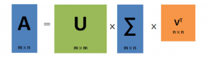
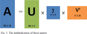
There is a method that can be applied to any matrix called Singular value decomposition (also known as VSD) can be used to accomplish this, Consider the following formula:

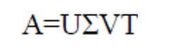
In this equation, “U” represents a matrix of the order mxm if “A” represents mxn ordered matrix. The vector of U matrix is orthogonal and called as left singular vector.  is a vector of mxn order matrix and VT is a transpose matrix of V in nxn order. The vector of the transpose of v represented as VT is also orthogonal and known as right singular vector.

 

 

Now, what’s the relationship in between eigenvalues and singular values? First and foremost, by multiplying a matrix let’s say A with its transpose matrix AT, we can obtain a square matrix. Now, using the formula    where V represents the right singular vectors, we can then compute the square matrix’s eigenvalues. Furthermore, we can obtain these variables:

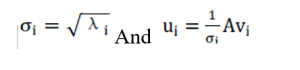
The variable u is the left singular vector, and the variable is the singular value mentioned above. To the eigenvalue of a matrix, the singular value is identical, except that the values in matrix are ordered from large to tiny and decreased very quickly.

The sum of 99 percent of singular values was accounted for by 10 percent or even 1 percent of single values in many cases. We may utilise the singular value of the previous r to roughly represent the matrix to put it another way and partial singular value decomposition can be described as follows:

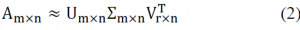
In comparison with m and n, r is a considerably smaller value.

Multiplying these three matrices on the right, yields a matrix that is close to A, where r is closer to n and the multiplication result is closer to A. The aggregate of the three matrix areas is substantially smaller than the original matrix A’s area (from the storage point of view, matrix area is smaller, storage size is smaller). So, we just need to save the three matrices

In order to represent the original matrix A in compressed space.

• Applications of SVD:

Following are some applications of singular value decomposition.

1. Singular value decomposition has been successfully used in signal processing to modify, analyse, and synthesise signals and sounds.
2. Singular value decomposition has useful application in face recognition and image processing using digital computer which uses different algorithms.

1. It can be used to determine non-scaled mode forms in face recognition, also known as model analysis.
2. Where mathematical models of the atmosphere are utilised to forecast weather based on current conditions, it is useful in numerical weather prediction.
3. In quantum information, where it is known as Schmidt decomposition, its relevance should not be neglected.

• Application in data analysis:

Even after how good the equipment is used or how well-designed the methodology is, there will always be some approximate measurements in the data we compute. The larger singular values correspond to the matrix’s principle information, as previously stated, making SVD an appropriate tool for data analysis.

• Experiment 1

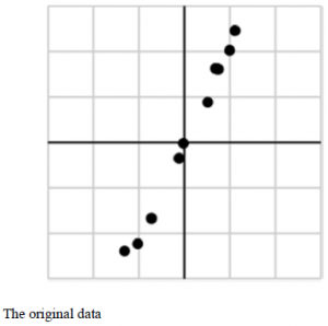
We obtained some data described in the above figure as an Experiment of SVD. Let’s give this data the matrix form:

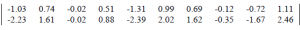
We get α1 and α2  after singular value decomposition. The corresponding values of the second singular values could be ignored and there are some noises in the datum since the first singular value is much larger than the second one.

The main sample points after the decomposition of SVD are shown in fig below:

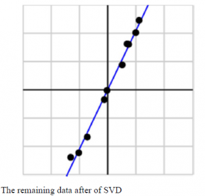
Principle component analysis also uses the Singular value decomposition to observe the values that depends on each other between rough data collected.

By observing the main sample datum that obtained, we believe that the process has some relation with principle component analysis.

• Comparison of PCA and SVD:

1. PCA is equal to approximating a factorized statement by keeping the largest terms and discarding all smaller terms, whereas SVD is straightly commensurate to factoring algebraic equations.
2. Principle component analysis is a machine intelligence method of determining the key characteristics, whereas Singular value decomposition values are constant numbers, and factorization is the process of dissecting them.
3. SVD is the breakdown of the matrix into orthonormal areas and although it is more expensive but PCA can be calculated using SVD.
4. In numerical linear algebra, SVD is a commonly used and multi-purpose data processing feature, whereas PCA is a well-developed method that has incorporated various statistical theories.
5. PCA is a dimensionality reduction technique while one of the most used methods is SVD.

• Conclusion:

Dimensionality reduction techniques like singular value decomposition (SVD) and principal component analysis (PCA) are commonly used in interpretation of the data analysis and Machine Learning. Both try to discover a linear collection of inputs in the initial high-dimensional data matrix in order to provide a representative picture of the database and both of them are typical linear dimensionality reduction algorithms.

Singular value decomposition with example

Various fields select them while dimensionality reduction.

Other Topics of Linear Algebra

• what are the row spaces, column spaces and null spaces in Linear Algebra?
• How to solve system of linear equations in Linear Algebra?
• what is the vector space in linear algebra? vector space example
• How to test the given vectors are linearly independent or not?
• What are the matrices and their types ?
• Finding Eigen Values and Eigen Vectors using MATLAB
• How to diagonalize a matrix? Example of diagonalization
• What are the shortcuts for finding the determinant of a matrix?
• What are the Block Matrices?
• what are the examples of scalar and vector quantities?
• How to perform similar matrices transformation?
• How to find the basis of a vector space V?
• what are the eigen values and eigen vectors? explain with examples
• What are the nodal incidence matrices?
• What is the application of linear algebra in cryptography?