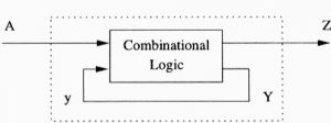
Sequential circuit
Discuss the Design Steps for Analysis of Asynchronous Sequential Circuits? Sequential Circuits are those in which the current output is dependent both on the current input and the previous output. It is a memory-equipped combinational circuit.

Asynchronous circuit
In contrast to synchronous circuits, asynchronous sequential circuits do not need clock signals. Instead, the circuit is driven by the input pulses, thus when the inputs change, the circuit’s state also changes. They don’t employ clock pulses either.
Design procedure
A number of steps must be made in order to simplify the circuit and produce a stable circuit devoid of important races. The steps in design are as follows, in brief:
- Create a simple flow table using the provided specification as a guide.
- The basic flow table’s rows are combined to decrease the flow table.
- Assign binary states variables to each row of the reduced flow table to produce the transition table.
- Assign output values to the dashes associated to the unstable states to produce the output mappings.
- Draw the logic diagram and make the excitation and output variables’ Boolean operations simpler.
The design process will be demonstrated using the following example:
Design Example – Specification
Make a gated latch circuit with Q as its sole output, G (gate), D (data), and both as its two inputs. A memory component called a gated latch accepts the value of D when G is 1 and holds onto it until G is 0. After G = 0, the value of the output Q is unaffected by changes in D.
Step 1: Primitive Flow Table
A primitive flow table is one that only has one stable total state in each row. The overall state is composed of the internal state and the input.
To derive the primitive flow table, a table describing all possible total states for the system is needed:
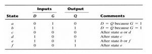
The resulting table produced by the gated latch is shown in the image below:
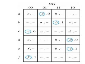
We then fill up one square in each row that represents the stable condition of the row.
Then, keeping in mind that both inputs cannot change at the same time, we enter dashes in each row that deviates by two or more variables from the input variables associated with the stable state.
The values for the extra two squares in each row are then determined. Using the comments from the previous table, it might be possible to find the needed data. Situations that don’t matter are denoted with a dash.
Step 2: Reduction of the Primitive Flow Table
The primitive flow table can be reduced to a smaller number of rows if two or more stable states are placed in the same row of the flow table. The streamlined merger rules are as follows:
- Two or more rows of the primitive flow table can be combined into one if there are no incompatible states and outputs in any of the columns.
- When one state symbol and entries marked “don’t care” are present in the same column, the state is listed in the merged row.
- If a state is circled in one of the rows, it gets circled in the combined row as well.
- The output state is also contained in each stable state in the merged row. Now apply these rules to the primitive flow table that was previously displayed.
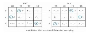
To illustrate how this is done, the fundamental flow table is split into two portions, each with three rows:

Each of the four columns indicates three stable states that can be joined because there aren’t any conflicting entries there. Because it indicates a don’t care condition, a dash can be attached to any state or output. It is possible to combine the output from the first column into the stable state c, the output from the second column into the stable state a, etc.
As a result, the flow table is smaller as follows:
Step 3: Transition Table and Logic Diagram
Each state needs to be assigned a binary value in order to create the circuit for the streamlined flow table. The flow table becomes a transition table as a result.
When allocating binary states, care must be taken to ensure that no circuit-critical races exist. It is impossible for a critical race to occur in a two-row flow table.
By assigning state a 0 and state b a 1, respectively, in the reduced flow table, the following transition table is produced:
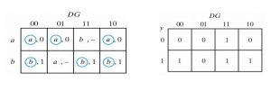
The transition table efficiently maps the excitation variable Y. The simplified Boolean function of the Y is, as seen from the map:
Y = DG +G′’y
Two outputs in the final reduced flow table have the designation “don’t care.” Assigning the values shown below to the output:

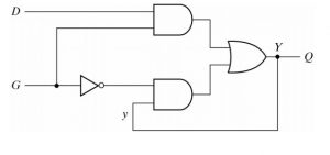
You can set the output Q to be equal to the output Y. If the outputs that don’t care are given the other possible values, output Q is equal to y. The logic diagram of the gated latch appears as follows:
4. REDUCTION OF STATE AND FLOW TABLES
Similar to how synchronous circuits are reduced in number of internal states, asynchronous sequential circuits adopt a similar technique.
5-Implication Table
The concept that two states in a state table can be combined into one if they can be proved to be equal forms the basis of the state-reduction technique for state tables that are completely described.
Sometimes two states will have equivalent next states even when they do not have the same next states.
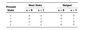
Consider the following state table:
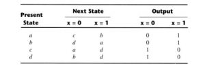
The statements (a, b) and (c, d) imply (a, b). Both sets of states are equivalent, i.e., both a and b and c and d are equivalent.
An implication table can be used to methodically check each pair of states in a table with several states for potential equivalence. This diagram is made up of squares—one for each potential pair of states—that have spaces for the possible implied states to be listed.

The implication table is:
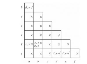
All of the states defined in the state table are listed, with the exception of the last, down the left side of the vertical list and across the bottom of the horizontal list, respectively.
States that are not equivalent are shown in the corresponding square with a “x,” while those that are equivalent are noted with a “.”
To identify whether or not the entries in some of the squares represent suggested states, more research must be done on them.
The step-by-step procedure of filling in the squares is as follows:
- Draw a cross in any square that represents a pair of states whose outputs do not match up with every input.
- Enter the pairs of states in the remaining squares that are implied by the pair of states shown in the squares. In order to accomplish that, we begin at the top square in the left column, go down, and then move on to the next column to the right.
- Go back and forth through the table to see if any more squares need to have a “x” placed next to them. If there is at least one inferred pair in the table that is not equal, that square is crossed out.
- The squares that do not have crosses are all checked off in the last step. These states are equivalent: (a, b), (d, e), (d, g) (e, g).
State pairs are now combined into larger groups of comparable states. Because each state in the group is equivalent to the other two, the final three pairs can be joined to form a set of three equivalent states (d, e, and g). The remaining states in the state table that are not equivalent to any other states are combined with the equivalent states identified from the implication table to form the final partition of these states:
(A, B, C, D, E, and G) (f)
The reduced state table is:
6-Merging of the Flow Table
The state table for a sequential circuit can occasionally be provided incorrectly.
The number of states in the flow table can be decreased by combining states with incomplete specifications. Such states cannot be compared to one another, however, it is claimed that they are compatible.
Three steps make up the procedure that must be used to identify an appropriate set of compatibles for the purpose of merging a flow table:
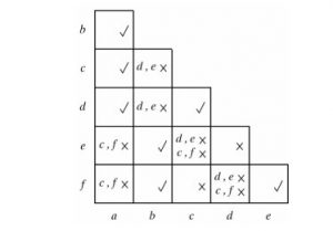
- Using the implication table, identify all couples that are compatible.
- Utilize a merger diagram to determine the greatest number of compatibles.
- Create a small, closed collection of compatibles that includes all the states.
The following simple flow table will be used to demonstrate and explain the three procedure steps:
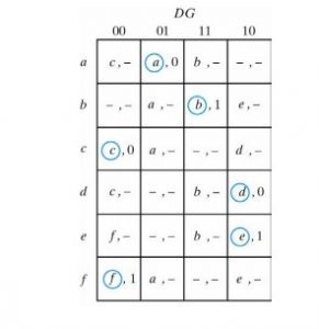
Compatible Pairs:
If there is no conflict in the output values and the two states are identical or compatible in every column of the corresponding rows in the flow table, they are said to be compatible.
These are the compatible pairs ():
a, b, c, d, e, f, c, d, a, d, b, e, and d, f (e, f)
RACE-FREE STATE ASSIGNMENT:
The basic goal of selecting an appropriate binary state assignment is to avoid crucial races.
When states where transitions occur in a flow table are assigned neighboring assignments, critical races are prevented. (For instance, 010 and 111 are close by.)
In a two-row flow table, there can never be a critical race.
Four-Row Flow Table Example:
Four-row flow tables need a minimum of two state variables.
Consider the following flow table and its corresponding transition diagram:
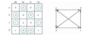
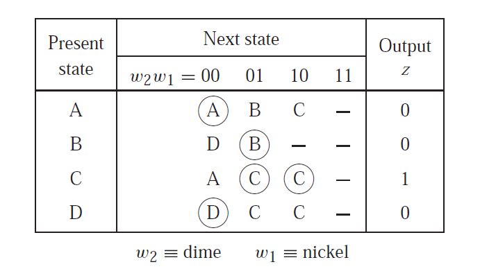
A state assignment map that is suitable for any four-row flow table is shown below:
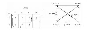
The initial states are a, b, c, and d; additional states are e, f, and g. By producing a cycle, the assignment makes guarantee that only one binary variable is changing at once.
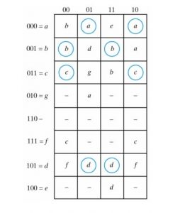
The four-row table can be expanded to a seven-row table that is free of critical races by using the assignment provided by the map:
Also read here
- How to design a 4 bit magnitude comparator circuit? Explanation with examples
- What is the magnitude comparator circuit? Design a 3 bit magnitude comparator circuit
- What are the synchronous counters? Explain with an example.
- what are the half adder and full adder circuits?
- what are the half subtractor and full subtractor circuits?
- How to design a four bit adder-subtractor circuit?
- What are number systems in computer?
- Discuss the binary counter with parallel load? Explain its working with an example
- how to draw state diagram of sequential circuit?
- How to simplify a Boolean function using Karnaugh map (k-map)?
- What are the flip flops and registers in digital design?
- Define fan-in, fan-out, CMOS and TTL logic levels
- what is the Canonical form representation of Boolean function?
- What is difference between latches and flip flops?