Table of Contents

Introduction

In this article we will Define Matrix Theory and Different Types of Matrixes. One of the most crucial thing in teachings of mathematics is “Matrix Theory and solution of its problems”. Matrix theory can assist researchers, practitioners, and peeps in solving a variety of problems in various fields like Engineering, Mathematics, Econometrics, Finance, Economics, optimization and decisional sciences and physics. In order to examine matrix theory with applications first we’ll discuss the theory of working. Than we will look on methods used in developing several mathematics, financial, economic and statistical models using some real life examples.

Finding roots of equation and system of equation are one of the most vital applications of matrix theory. In 1967, Butle presented a solution of coupled equation using R- matrix technique and EL-sayed and Ran showed an iteration method to solve various classes of non-linear matrix equations. In 2010, a new operational matrix was introduced to solve fractional order equation. Doha proposed Jacobi transformation for order differential equations. The operational matrix is used to simplify fractional differential equation.

Matrix theory is important in a variety of scientific researches. It have been used in different areas of Physics, including classical mechanics, optics and quantum mechanics. The study of matrices also been used to investigate few physical phenomena, such as motion of rigid bodies. Also, in computers graphics have been used for developing 3-D models and projecting them on onto 2-D surfaces.

Stochastic matrices tell how to show the set of probabilities in probability theory and statistics. The calculations of matrix are being used in traditional analytical concepts such as derivatives and exponential functions (higher dimensional function). Furthermore, matrices can be used in economics to depict economic relationships. Schott (2016) introduced the matrix analysis test statistics to discover physiologically relevant changes. Magnus and Neudeker created matrix differential calculus with applications in statistical and econometrical applications.

Review of matrix theory

In this section, we give definitions of matrix and some common types of matrices.

Definition

A matrix is a rectangular array in math that holds numbers, symbols, or phrases in columns and rows according to some specified rules and regulations.

An element or item is the name given to each cell in a matrix.

For instance, consider a matrix M of 2 rows and 2columns and a matrix N with 3 rows and 3 columns

When the number of column and rows are equal to each other, such matrices are called square matrix.

Types of matrices

Null matrix

A matrix whose all entries are zero is commonly known as a null matrix or zero matrix.

For instance,

\begin{equation}
M=\left[\begin{array}{llllll}
0 & 0 & 0 & 0 & 0 & 0
\end{array}\right]
\end{equation}

Identity matrix

An identity matrix is a diagonal matrix with all diagonal members equal to one. That’s mii =1. The dimensions can be specified using I or E.

Let’s see an example:

\begin{equation}
\mathrm{M}=\left[\begin{array}{llll}
1 & 0 & 0 & 1
\end{array}\right] \text { and }\left[\begin{array}{lllllllll}
1 & 0 & 0 & 0 & 1 & 0 & 0 & 0 & 1
\end{array}\right]
\end{equation}

Diagonal matrix

A square matrix in which all the entries outside the diagonal is equal to 0 is called diagonal matrix. They are usually represented as mij =0.

For example:

Inverse of a matrix

If M is a square matrix of dimension n, than N is an inverse matrix of M if MN=NM=I, where I represents an identity matrix. Only if M has an inverse than the matrix can be said as invertible matrix.

For instance,

\begin{equation}
\mathrm{M}=\left[\begin{array}{llll}
4 & 3 & 2 & 1
\end{array}\right] \text { and } \mathrm{N}=[-0.511 .5-2] \text {, than } \mathrm{MN}=\mathrm{NM}=\mathrm{I}
\end{equation}

Transpose of a matrix

When we switch the rows with columns and columns with rows of a matrix M it is called as transpose of a matrix M.

For instance:

\begin{equation}
\text { Matrix } M=\left[\begin{array}{llllll}
1 & 2 & 4 & 4 & 3 & 3
\end{array}\right], \text { transpose } M^{t}=\left[\begin{array}{llllll}
1 & 4 & 2 & 3 & 4 & 3
\end{array}\right]
\end{equation}

Conjugate transpose matrix

If M is a m*n matrix containing entries from a field F, the conjugate transpose of M is found first by computing complex conjugate of each entry M and transpose of matrix M. A matrix of conjugate transposes M=(mij) usually shown as = M*.

For example:

If $\mathrm{M}=[1-2 i 1-3 i 433+2 i]$ than $\mathrm{M}=[12 i 1+3 i 433-2 i]$ and
$$
M^{T}=\mathrm{M}^{*}=[11+3 i 32 i 43-2 i]
$$

Thus M is a conjugate transpose matrix.

Orthogonal matrix

A matrix is called as orthogonal if M= M=I , where M is a matrix , is transpose of a matrix M and I symbolizes Identity . It shows equivalent equality, M is orthogonal matrix only when its inverse is equal to the transpose of a matrix M.

$$
M^{-1}=M^{T}
$$
For instance:
$$
\mathrm{M}=\left[\begin{array}{llll}
0 & 1 & 1 & 0
\end{array}\right] \text { is } M^{-1}=M^{T}=\left[\begin{array}{llll}
1 & 0 & 0 & 1
\end{array}\right]
$$

Unitary matrix

M is referred as unitary matrix only if M*M=I, where I shows an identity matrix and M gives unitary matrix also M* is a transpose conjugate. When the inverse of a matrix equals its conjugate transpose , than its said to be an orthogonal matrix it should prove =\begin{equation}
M^{-1}=M^{T}
\end{equation}

$\mathrm{I}=\operatorname{Det}(\mathrm{I})=\operatorname{Det}\left(\mathrm{M}^{*} \mathrm{M}\right)=\operatorname{Det}\left(\mathrm{M}^{*}\right) \operatorname{Det}(\mathrm{M})=[\operatorname{Det}(\mathrm{M})]^{\text {square }}$
For instance,
$$
\begin{aligned}
&\mathrm{M}=[1+i / 2-1+i / 21+i / 21-i / 2], \mathrm{M}=[1-i / 2-1-i / 2 \overline{1}-i / 21+i / 2] \text { and } \\
&\mathrm{M}^{*}=M^{T}
\end{aligned}
$$
Hence, $M$ is a unitary matrix.

Symmetric matrix

When a matrix and its transpose M^Tare same, it indicates that the matrix is symmetric.

Let’s see an example.

\begin{equation}
M=\left[\begin{array}{llll}
2 & 5 & 5 & 2
\end{array}\right] \text { is equal to its transpose } M^{T}=\left[\begin{array}{llll}
2 & 5 & 5 & 2
\end{array}\right]
\end{equation}

So it is a symmetric matrix.
* Hermitian matrix:
A matrix is said to be Hermitian if $\mathrm{M}=M^{T}$. For easier to understand let’s look below $\mathrm{M}=[13+2 i 3-2 i 4], \mathrm{M}=[13-2 i 3+2 i 4]$ and $M^{T}=[13+2 i 3-2 i 4]$
It’s a Hermitian matrix.

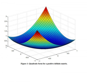
*ositive definite matrix:
A hermitian matrix is called as PSD (positively semi definite) if $u^{t} \mathrm{Mu}>0$, where $u$ is not equal to zero. For better understanding consider the following example.

If $\mathrm{M}=\left[\begin{array}{llll}7 & 0 & 0 & 9\end{array}\right]$ and $u^{t} \mathrm{Mu}=(\mathrm{u} 1 \mathrm{u} 2)\left[\begin{array}{lll}7 & 0 & 0\end{array}\right][u 1 u 2]=7 u 1^{2}+9 u 2^{2}>=0$. Then, $\mathrm{M}$ can be said to be a positive definite matrix

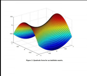
Indefinite matrix

A Hermitian matrix that is not PSD or PD is known as indefinite matrix. The explanation for an indefinite matrix of the quadratic form is given.

$$
\mathrm{M}=\left[\begin{array}{llll}
2 & 0 & 0 & -3
\end{array}\right] \text { and } u^{t} \mathrm{Mu}=(\mathrm{u} 1 \mathrm{u} 2)\left[\begin{array}{llll}
2 & 0 & 0 & -3
\end{array}\right][u 1 u 2]=2 u 1^{2}-3 u 2^{2} \text {. }
$$
It shows $M$ is an indefinite form of the matrix.